Fitness – Science4Performance

Strava Power Curve

Screen Shot 2018-05-11 at 16.34.08 — Comparing Historic Power Curves

If you use a power meter on Strava premium, your Power Curve provides an extremely useful way to analyse your rides. In the past, it was necessary to perform all-out efforts, in laboratory conditions, to obtain one or two data points and then try to estimate a curve. But now your power meter records every second of every ride. If you have sustained a number of all-out efforts over different time intervals, your Power Curve can tell you a lot about what kind of rider you are and how your strengths and weaknesses are changing over time.

Strava provides two ways to view your Power Curve: a historical comparison or an analysis of a particular ride. Using the Training drop-down menu, as shown above, you can compare two historic periods. The curves display the maximum power sustained over time intervals from 1 second to the length of your longest ride. The times are plotted on a log scale, so that you can see more detail for the steeper part of the curve. You can select desired time periods and choose between watts or watts/kg.

The example above compares this last six weeks against the year to date. It is satisfying to see that the six week curve is at, or very close to, the year to date high, indicating that I have been hitting new power PBs (personal bests) as the racing season picks up. The deficit in the 20-30 minute range indicates where I should be focussing my training, as this would be typical of a breakaway effort. The steps on the right hand side result from having relatively few very long rides in the sample.

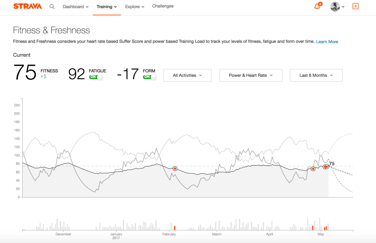
Note how the Power Curve levels off over longer time periods: there was a relatively small drop from my best hour effort of 262 watts to 243 watts for more than two hours. This is consistent with the concept of a Critical Power that can be sustained over a long period. You can make a rough estimate of your Functional Threshold Power by taking 95% of your best 20 minute effort or by using your best 60 minute effort, though the latter is likely to be lower, because your power would tend to vary quite a bit due to hills, wind, drafting etc., unless you did a flat time trial. Your 60 minute normalised power would be better, but Strava does not provide a weighted average/normalised power curve. An accurate current FTP is essential for a correct assessment of your Fitness and Freshness.

Switching the chart to watts/kg gives a profile of what kind of rider you are, as explained in this Training Peaks article. Sprinters can sustain very high power for short intervals, whereas time trial specialists can pump out the watts for long periods. Comparing myself against the performance table, my strengths lie in the 5 minutes to one hour range, with a lousy sprint.

Screen Shot 2018-05-11 at 17.19.45.png — Single Ride Power Curve versus Historic

The other way to view your Power Curve comes under the analysis of a particular ride. This can be helpful in understanding the character of the ride or for checking that training objectives have been met. The target for the session above was to do 12 reps on a short steep hill. The flat part of the curve out to about 50 seconds represents my best efforts. Ideally, each repetition would have been close to this. Strava has the nice feature of highlighting the part of the course where the performance was achieved, as well as the power and date of the historic best. The hump on the 6-week curve at 1:20 occurred when I raced some club mates up a slightly longer steep hill.

If you want to analyse your Power Curve in more detail, you should try Golden Cheetah. See other blogs on Strava Fitness and Freshness, Strava Ride Statistics or going for a Strava KOM.

Kings and Queens of the Mountains

Screen Shot 2017-11-09 at 18.40.09.png

I guess that most male cyclists don’t pay much attention to the women’s leaderboards on Strava. And if they do it might just be to make some puerile remark about boys being better than girls. From a scientific perspective the comparison of male and female times leads to some interesting analysis.

Assuming both men and women have read my previous blogs on choosing the best time, weather conditions and wind directions for the segment that suits their particular strengths, we come back to basic physics.

KOM or QOM time = Work done / Power = (Work against gravity + Drag x Distance + Rolling resistance x Distance) / (Mass x Watt/kg)

Of the three components of work done, rolling resistance tends to be relatively insignificant. On a very steep hill, most of the work is done against gravity, whereas on a flat course, aerodynamic drag dominates.

The two key factors that vary between men and women are mass and power to weight ratio (watts per kilo). A survey published by the ONS in 2010, rather shockingly reported that the average British man weighed 83.6kg, with women coming in at 70.2kg. This gives a male/female ratio of 1.19. KOM/QOM cyclists would tend to be lighter than this, but if we take 72kg and 60kg, the ratio is still 1.20.

Males generate more watts per kilogram due to having a higher proportion of lean muscle mass. Although power depends on many factors, including lungs, heart and efficiency of circulation, we can estimate the relative power to weight ratio by comparing the typical body composition of males and females. Feeding the ONS statistics into the Boer formula gives a lean body mass of 74% for men and 65% for women, resulting in a ratio of 1.13. This can be compared against the the useful table on Training Peaks showing maximal power output in Watts/kg, for men and women, over different time periods and a range of athletic abilities. The table is based on the rows showing world record performances and average untrained efforts. For world champion five minute efforts and functional threshold powers, the ratios are consistent with the lean mass ratio. It makes sense that the ratio should be higher for shorter efforts, where the male champions are likely to be highly muscular. Apparently the relative performance is precisely 1.21 for all durations in untrained people.

Screen Shot 2017-11-08 at 10.23.33

On a steep climb, where the work done against gravity dominates, the benefit of additional male muscle mass is cancelled by the fact that this mass must be lifted, so the difference in time between the KOM and the QOM is primarily due to relative power to weight ratio. However, being smaller, women suffer from the disadvantage that the inert mass of bike represents a larger proportion of the total mass that must be raised against gravity. This effect increases with gradient. Accounting for a time difference of up to 16% on the steepest of hills.

In contrast, on a flat segment, it comes down to raw power output, so men benefit from advantages in both mass and power to weight ratio. But power relates to the cube of the velocity, so the elapsed time scales inversely with the cube root of power. Furthermore, with smaller frames, women present a lower frontal area, providing a small additional advantage. So men can be expected to have a smaller time advantage of around 9%. In theory the advantage should continue to narrow as the gradient shifts downhill.

Theory versus practice

Strava publishes the KOM and QOM leaderboards for all segments, so it was relatively straightforward to check the basic model against a random selection of 1,000 segments across the UK. All leaderboards included at least 1,666 riders, with an overall average of 637 women and 5,030 men. One of the problems with the leaderboards is that they can be contaminated by spurious data, including unrealistic speeds or times set by groups riding together. To combat this, the average was taken of the top five times set on different dates, rather than simply to top KOM or QOM time.

The average segment length was just under 2km, up a gradient of 3%. The following chart plots the ratio of the QOM time to the KOM time versus gradient compared with the model described above. The red line is based on the lean body mass/world record holders estimate of 1.13, whereas the average QOM/KOM ratio was 1.32. Although there is a perceivable upward slope in the data for positive gradients, clearly this does not fit the data.

Screen Shot 2017-11-09 at 17.54.43

Firstly, the points on the left hand side indicate that men go downhill much more fearlessly than women, suggesting a psychological explanation for the observations deviating from the model. To make the model fit better for positive gradients, there is no obvious reason to expect the weight ratio of male to female Strava riders to deviate from the general population, so this leaves only the relative power to weight ratio. According to the model the QOM/KOM ratio should level off to the power to weight ratio for steep gradients. This seems to occur for a value of around 1.40, which is much higher than the previous estimates of 1.13 or the 1.21 for untrained people. How can we explain this?

A notable feature of the data set was that sample of 1,000 Strava segments was completed by nearly eight times as many men as women. This, in turn reflects the facts that there are more male than female cyclists in the UK and that men are more likely to upload, analyse, publicise and gloat over their performances than women.

Having more men than women, inevitably means that the sample includes more high level male cyclists than equivalent female cyclists. So we are not comparing like with like. Referring back to the Training Peaks table of expected power to weight ratios, a figure of 1.40 suggests we are comparing women of a certain level against men of a higher category, for example, “very good” women against “excellent” men.

A further consequence of having far more men than women is that is much more likely that the fastest times were recorded in the ideal conditions described in my previous blogs listed earlier.

Conclusions

There is room for more women to enjoy cycling and this will push up the standard of performance of the average amateur rider. This would enhance the sport in the same way that the industry has benefited as more women have joined the workforce.

Strava Fitness and Freshness

The last blog explored the statistics that Strava calculates for each ride. These feed through into the Fitness & Freshness chart provided for premium users. The aim is to show the accumulated effect of training through time, based on the Training-Impulse model originally proposed by Eric Banister and others in a rather technical paper published in 1976.

Strava gives a pretty good explanation of Fitness and Freshness. A similar approach is used on Training Peaks in its Performance Management Chart. On Strava, each ride is evaluated in terms of its Training Load, if you have a power meter, or a figure derived from your Suffer Score, if you just used a heart rate monitor. A training session has a positive impact on your long-term fitness, but it also has a more immediate negative effect in terms of fatigue. The positive impact decays slowly over time, so if you don’t keep up your training, you lose fitness. But your body is able to recover from fatigue more quickly.

The best time to race is when your fitness is high, but you are also sufficiently recovered from fatigue. Fitness minus fatigue provides an estimate of your form. The 1976 paper demonstrated a correlation between form and the performance of an elite swimmers’ times over 100m.

The Fitness and Freshness chart is particularly useful if you are following a periodised training schedule. This approach is recommended by many coaches, such as Joe Friel. Training follows a series of cycles, building up fitness towards the season’s goals. A typical block of training includes a three week build-up, followed by a recovery week. This is reflected in a wave-like pattern in your Fitness and Freshness chart. Fitness rises over the three weeks of training impulses, but fatigue accumulates faster, resulting in a deterioration of form. However, fatigue drops quickly, while fitness is largely maintained during the recovery week, allowing form to peak.

In order to make the most of the Fitness and Freshness charts, it is important that you use an accurate current figure for your Functional Threshold Power. The best way to do this is to go and do a power test. It is preferable to follow a formal protocol that you can repeat, such as that suggested by British Cycling. Alternatively, Strava premium users can refer to the Strava Power Curve. You can either take your best effort over 1 hour or 95% of your best effort over 20 minutes. Or you can click on the “Show estimated FTP” button and take the lower figure. In order for this to flow through into your Fitness and Freshness chart, you need to enter your 1 hour FTP into your personal settings, under “My Performance”.

The example chart at the top of this blog shows how my season has panned out so far. After taking a two week break before Christmas, I started a solid block of training in January. My recovery week was actually spent skiing (pretty hard), though this did not register on Strava because I did not use a heart rate monitor. So the sharp drop in fatigue at the end of January is exaggerated. Nevertheless, my form was positive for my first race on 4 February. Unfortunately, I was knocked off and smashed a few ribs, forcing me to take an unplanned two week break. By the time I was able to start riding tentatively, rather than starting from an elevated level, my fitness had deteriorated to December’s trough.

After a solid, but still painful, block of low intensity training in March, I took another “recovery week” on the slopes of St Anton. I subsequently picked up a cold that delayed the start of the next block of training, but I have incorporated some crit races into my plan, for higher intensity sessions. If you edit the activity and make the “ride type” a “race”, it shows up as a red dot on the chart. Barring accident and illness, the hope is to stick more closely to a planned four-week cycle going forward.

This demonstrates how Strava’s tools reveal the real-life difficulties of putting the theoretical benefits of periodisation into practice.

Modelling Strava Fitness and Freshness

Supercompensating with Strava

See other blogs on Strava Power Curve, Strava Ride Statistics or going for a Strava KOM.

Tag: Fitness