Milan Sanremo in a Random Forest

Last time I tried to predict a race, I trained up a neural network on past race results, ahead of the World Championships in Harrogate. The model backed Sam Bennett, but it did not take account of the weather conditions, which turned out to be terrible. Fortunately the forecast looks good for tomorrow’s Milan Sanremo.

This time I have tried using a Random Forest, based on the results of the UCI races that took place in 2020 and so far in 2021. The model took account of each rider’s past results, team, height and weight, together with key statistics about each race, including date, distance, average speed and type of parcours.

One of the nice things about this type of model is that it is possible to see how the factors contribute to the overall predictions. The following waterfall chart explains why the model uncontroversially has Wout van Aert as the favourite.

Breakdown of prediction for Wout van Aert

The largest positive contribution comes from being Wout van Aert. This is because he has a lot of good results. His height and weight favour Milan Sanremo. He also has a strong positive coming from his team. This distance and race type make further positive contributions.

We can contrast this with the model’s prediction for Mathieu van der Poel, who is ranked 9th.

Breakdown of prediction for Mathieu van der Poel

We see a positive personal contribution from being van der Poel, but having raced fewer UCI events, he has less of a strong set of results than van Aert. According to the model the Alpecin Fenix team contribution is not a strong as Jumbo Visma, but the long distance of the race works in favour of the Dutchman. The day of year gives a small negative contribution, suggesting that his road results have been stronger later in the year, but this could be due to last year’s unusual timing of races.

Each of the other riders in the model’s top 10 is in with a shout.

It’s taken me all afternoon to set up this model, so this is just a short post.

Post race comment

Where was Jasper Stuyven?

Like Mads Pedersen in Harrogate back in 2019, Jasper Stuyven was this year’s surprise winner in Sanremo. So what had the model expected for him? Scrolling down the list of predictions, Stuyven was ranked 39th.

Breakdown of prediction for Jasper Stuyven

His individual rider prediction was negative, perhaps because he has not had many good results so far this year, though he did win Omloop Het Nieuwsblad last year and had several top 10 finishes. The model assessed that his greatest advantage came from the length of the race, suggesting that he tends to do well over greater distances.

The nice thing about this approach is that that it identifies factors that are relevant to particular riders, in a quantitative fashion. This helps to overcome personal biases and the human tendency to overweight and project forward what has happened most recently.

Pro cycling team networks

The COVID-19 pandemic has further exposed the weakness of the professional cycling business model. The competition between the teams for funding from a limited number of sponsors undermines the stability of the profession. With marketing budgets under strain, more teams are likely to face difficulties, in spite of the great advertising and publicity that the sport provides. Douglas Ryder is fighting an uphill struggle trying to keep his team alive after the withdrawal of NTT as a lead sponsor. One aspect of stability is financial, but another measure is the level of transfers between teams.

The composition of some teams is more stable than others. This is illustrated by analysing the history of riders’ careers, which is available on ProCyclingStats. The following chart is a network of the transfers between teams in the last year, where the yellow nodes are 2020 teams and the purple ones are 2019. The width of the edges indicates how many riders transferred between the teams, with the thick green lines representing the bulk of the riders who stuck with the same team. The blue labels give the initials of the official name of each team, such as M-S (Mitchelton-Scott), MT (Movistar Team), T-S (Trek-Segafredo) and TS (Team Sunweb). Riders who switched teams are labelled in red.

Although there is a Dutch/German grouping on the lower right, the main structure is from the outside towards the centre of the network.

The spikes around the end of the chart show riders like Geoffrey Soupe or Rubén Fernández, who stepped down to smaller non World Tour teams like Team Total Direct Energie (TTDE), Nippo Delko One Provence (NNDP), Euskaltel-Euskadi (E-E), Androni Giocattoli-Sidermec (AG-S ) or U-XPCT (Uno-X Pro Cycling Team).

The two World Tour outliers were Mitchelton-Scott (M-S) and Groupama FDJ (GF), who retained virtually all their riders from 2019. Moving closer in, a group of teams lies around the edge of the central mass, where a few transfers occurred. Moving anti-clockwise we see CCC Team (CT), Astana Pro Team (APT), Trek-Segafredo (T-S), AG2R Le Mondial (ALM), Circus-Wanty Gobert (C-WG), Team Jumbo Visma (TJV), Bora-Hansgrohe (B-H) and EF Pro Cycling (EPC).

Deeper in the mêlée, Ineos (TI_19/IG_20), Deceuninck – Quick Step (D-QS), UAE-Team Emirates (U-TE), Lotto Soudal (LS), Bahrain – McLaren (B-H) and Movistar Team(MT) exchanged a number of riders.

Right in the centre Israel Start-Up Nation (IS-UN) grabbed a whole lot of riders, including 7 from Team Arkéa Samsic (TAS). Meanwhile likes of Victor Campenaerts and Domenico Pozzovivo are probably regretting joining NTT Pro Cycling (TDD_19/NPC_20).

Looking forward

A few of the top riders have contracts for next year showing up on ProCyclingStats. So far 2020/2021 looks like the network below. Many riders are renewing with their existing teams, indicated by the broad green lines. But some big names are changing teams, including Chris Froome, Richie Porte, Laurens De Plus, Sam Oomen, Romain Bardet and Wilco Keldeman, Bob Jungels and Lilian Calmejane.

What about networks of riders?

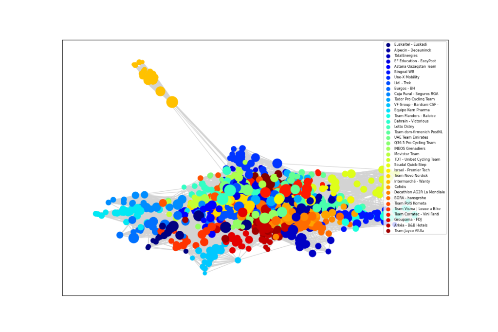
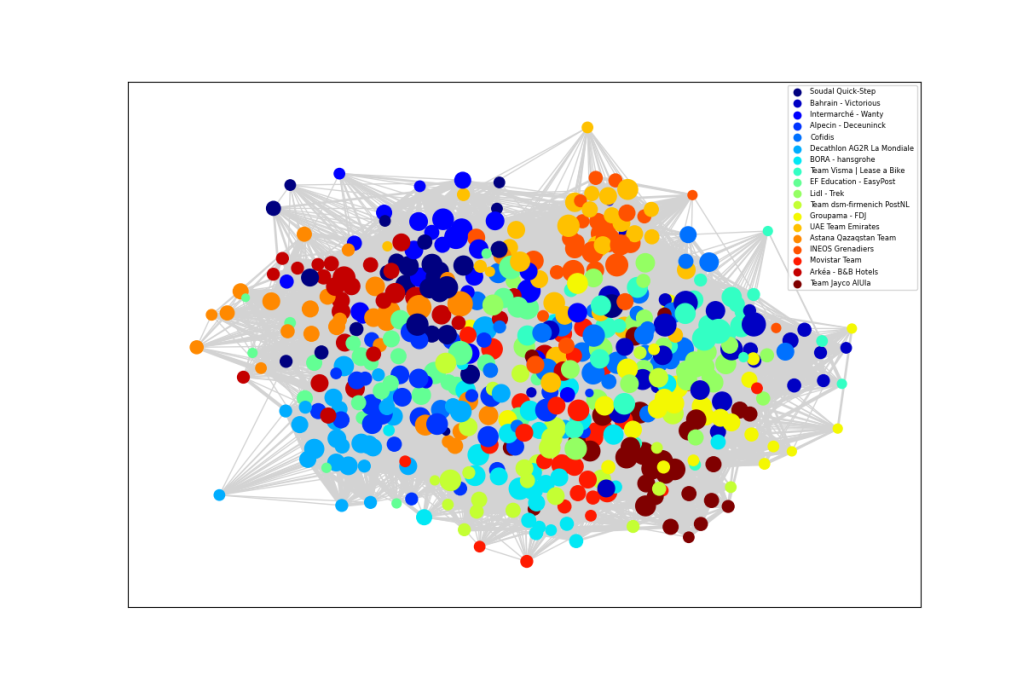
My original thought when starting this analysis was that over their careers, certain riders must have been team mates with most of the riders in today’s peloton, so who is the most connected? Unfortunately this turned out to be ridiculously complicated, as shown in the image below, where nodes are riders with links if they were ever teammates and the colours represent the current teams. The highest ranked rider in each team is shown in red.

It is hard to make much sense of this, other than to note that those with shorter careers in the same team are near the edge and that Philippe Gilbert is close to the centre. Out of interest, the rider around 9 o’clock linking Bora and Jumbo Visma is Christoph Pfingsten, who moved this year. At least we can conclude that professional cyclists are well-connected.

Time to be aerodynamic

The Covid-19 epidemic provided a huge boost to the Zwift streaming service. Confined by a global lockdown, cyclists freed themselves from the boredom of pedalling on a static turbo trainer by logging into one of a broadening range of online virtual worlds. Zwift racing has become particularly popular. While it is relatively straightforward to simulate variations in gradient and even the effects of drafting, it is not possible for riders to demonstrate superior bike handling skills. Nor can racers benefit from adopting a superior aerodynamic position on the bike, in fact this may prove to be a disadvantage.

Setting aside e-doping suspicions, such as riders understating their weights, in the artificial world of a Zwift race, the outcome largely comes down the the ability to sustain a high level of power (watts per kilo). The engagingly competitive nature of simulated races encourages everyone to push their limits. However, since Zwift offers no penalty against maintaining a non-aerodynamic body position on your trainer, it is quite possible that regular Zwifters might become habituated to riding in position that is far from optimal for the road.

Fresh aerodynamics

Once out in the fresh air again, many riders may have noticed improvements in the levels of power they are able to sustain, thanks to the high levels of exertion required to compete on Zwift. But in the real world, when it comes to beating other riders in a race or a time trial, the principle force a rider has to overcome is aerodynamic drag, not electromagnetic resistance.

Maximum speed is attained by adopting a riding position that provides the optimal tradeoff between the ability to generate power and a low level of aerodynamic drag. Drag depends on a rider’s CdA, which represents the drag coefficient multiplied by frontal area. Since power rises with the cube of velocity, there comes a point where it is better to compromise on power in order to reduce frontal area. This is the key to time trialing and successful breakaways.

When the race season begins, skilful and more aerodynamic racers will be able to benefit from drafting in the huge wind shadow created by Zwift diesels, while offering back much less assistance when they pull through. So after prolonged training on Zwift, racers and time trialists really need to focus on improving their aerodynamics

There are various ways to reduce drag, starting withs some basics as described in an earlier blog. Post ride analysis can be performed using Golden Cheetah, BestBikeSplit or MyWindSock. There is also a range of devices that claim to offer real time measurement of CdA. These have been primarily targeted at the TT/triathlon market, but there’s no doubt that these could be incredibly useful for both training or even, perhaps, a race breakaway. Cycling Weekly recently reviewed the Notio device, but, while useful, these tools remain expensive and a bit clunky.

Whatever you choose to do, stay safe and stay aero.

No drafting

In a fascinating white paper, Bert Blocken, Professor of Civil Engineering at Eindhoven University of Technology, comments on social distancing when applied to walking, running or cycling. His point is that the government recommendations to maintain a distance of 1.5 or 2 metres assume people are standing still indoors or outdoors in calm weather. However, when a person is moving, the majority of particulate droplets are swept along in a trailing slipstream.

Cyclists typically prefer to ride closely behind each other, in order to benefit from the aerodynamic drafting effect. Cycling is currently a permitted form of exercise in the UK, though only if riding alone or with members of your household. Nevertheless, there may be times when you find yourself catching up with a cyclist ahead. In this situation, you should avoid the habitual tendency to move up into the slipstream of the rider in front.

Professor Blocken’s team has performed computational fluid dynamics (CFD) simulations showing the likely spread of micro-droplets behind people moving at different speeds. As the cloud of particles, produced when someone coughs or sneezes, is swept into the slipstream, the heavier droplets, shown in red in the diagram above, fall faster. These are generally thought to be more considerably more contagious. You can see that they can land on the hands and body of the following athlete.

Based on the results, Blocken advises to keep a distance of at least four to five meters behind the leading person while walking in the slipstream, ten meters when running or cycling slowly and at least twenty metres when cycling fast.

Social Distancing v2.0

The recommendation, for overtaking other cyclists, is to start moving into a staggered position some twenty metres behind the rider in front, consistently avoiding the slipstream as you pass.

The results will be reported in a forthcoming peer-reviewed publication. But given the importance of the topic, I recommend that you take a look at the highly accessible three page white paper available here.

References

Social Distancing v2.0: During Walking, Running and Cycling
Bert Blocken, Fabio Malizia, Thijs van Druenen, Thierry Marchal

Bike Identification as a web app

One of the first skills acquired in the latest version of the fast.ai course on deep learning is how to create a production version of an image classifier that runs as a web application. I decided to test this out on a set of images of road bikes, TT bikes and mountain bikes. To try it out, click on the image above or go to this website https://bike-identifier.onrender.com/ and select an image from your device. If you are using a phone, you can try taking photos of different bikes, then click on Analyse to see if they are correctly identified. Side-on images work best.

How does it work?

The first task was to collect some sample images for the three classes of bicycles I had chosen: road, TT and MTB. It turns out that there is a neat way to obtain the list of urls for a Google image search, by running some javascript in the console. I downloaded 200 images for each type of bike and removed any that could not be opened. This relatively small data set allowed me to do all the machine learning using the CPU on my MacBook Pro in less than an hour.

The fast.ai library provides a range of convenient ways to access images for the purpose of training a neural network. In this instance, I used the default option of applying transfer learning to a pre-trained ResNet34 model, scaling the images to 224 pixel squares, with data augmentation. After doing some initial training, it was useful to look at the images that had been misclassified, as many of these were incorrect images of motorbikes or cartoons or bike frames without wheels or TT bars. Taking advantage of a useful fast.ai widget, I removed unhelpful training images and trained the model further.

The confusion matrix showed that final version of my model was running at about 90% accuracy on the validation set, which was hardly world-beating, but not too bad. The main problem was a tendency to mistake certain road bikes for TT bikes. This was understandable, given the tendency for road bikes to become more aero, though it was disappointing when drop handlebars were clearly visible.

The next step was to make my trained network available as a web application. First I exported the models parameter settings to Dropbox. Then I forked a fast.ai repository into my GitHub account and edited the files to link to my Dropbox, switching the documentation appropriately for bicycle identification. In the final step, I set up a free account on Render to host a web service linked to my GitHub repository. This automatically updates for any changes pushed to the repository.

Amazingly, it all works!

References

fast.ai lesson 2

My GitHub repository, include Jupyter notebook

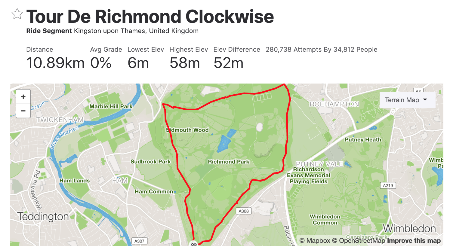
Strava – Tour de Richmond Park Clockwise

Screenshot 2019-05-22 at 15.24.51

Following my recent update on the Tour de Richmond Park leaderboard, a friend asked about the ideal weather conditions for a reverse lap, clockwise around the park. This is a less popular direction, because it involves turning right at each mini-roundabout, including Cancellara corner, where the great Swiss rouleur crashed in the 2012 London Olympics, costing him a chance of a medal.

An earlier analysis suggested that apart from choosing a warm day and avoiding traffic, the optimal wind direction for a conventional anticlockwise lap was a moderate easterly, offering a tailwind up Sawyers Hill. It does not immediately follow that a westerly wind would be best for a clockwise lap, because trees, buildings and the profile of the course affect the extent to which the wind helps or hinders a rider.

Currently there are over 280,000 clockwise laps recorded by nearly 35,000 riders, compared with more than a million anticlockwise laps by almost 55,000 riders. As before, I downloaded the top 1,000 entries from the leaderboard and then looked up the wind conditions when each time was set on a clockwise lap.

In the previous analysis, I took account of the prevailing wind direction in London. If wind had no impact, we would expect the distribution of wind directions for leaderboard entries to match the average distribution of winds over the year. I defined the wind direction advantage to be the difference between these two distributions and checked if it was statistically significant. These are the results for the clockwise lap.

RoseSegmentBarSegmentclockwise

The wind direction advantage was significant (at p=1.3%). Two directions stand out. A westerly provides a tailwind on the more exposed section of the park between Richmond Gate and Roehampton, which seems to be a help, even though it is largely downhill. A wind blowing from the NNW would be beneficial between Roehampton and Robin Hood Gate, but apparently does not provide much hindrance on the drag from Kingston Gate up to Richmond, perhaps because this section of the park is more sheltered. The prevailing southwesterly wind was generally unfavourable to riders setting PBs on a clockwise lap.

The excellent mywindsock web site provides very good analysis for avid wind dopers. This confirms that the wind was blowing predominantly from the west for the top ten riders on the leaderboard, including the KOM, though the wind strength was generally light.

The interesting thing about this exercise is that it demonstrates a convergence between our online and our offline lives, as increasing volumes of data are uploaded from mobile sensors. A detailed analysis of each section of the million laps riders have recorded for Richmond Park could reveal many subtleties about how the wind flows across the terrain, depending on strength and direction. This could be extended across the country or globally, potentially identifying local areas where funnelling effects might make a wind turbine economically viable.

References

Jupyter notebook for calculations

Can self-driving cars detect cyclists?

Screenshot 2019-05-10 at 14.05.59

Self-driving cars employ sophisticated software to interpret the world around them. How do these systems work? And how good are they at detecting cyclists? Can cyclists feel safe sharing roads with an increasing number of vehicles that make use of these systems?

How hard is it to spot a cyclist?

Vehicles can use a range of detection systems, including cameras, radar and lidar.  Deep learning techniques have become very good at identifying objects in photographic images. So one important question is how hard is it to spot a cyclist in a photo taken from a moving vehicle?

Researchers at Tsinghua University, working in collaboration with Daimler, created a publicly available collection of dashboard camera photos, where humans have painstakingly drawn boxes around other road users. The data set is used by academics to benchmark the performance of their image recognition algorithms. The images are rather grey and murky, reflecting the cloudy and polluted atmosphere of the Chinese city location. It is striking that, in the majority of cases, the cyclists are very small, representing around 900 pixels out of the 2048 x 1024 images, i.e. less than 0.05% of the total area. For example, the cyclist in the middle of the image above is pretty hard to make out, even for a human.

Object-detecting neural networks are typically trained to identify the subject of a photo, which normally takes up are significant portion of the image. Finding a tall, thin segment containing a cyclist is significantly more difficult.

If you think about it, the cyclist taking up the largest percentage of a dash cam image will be riding across the direction of travel, directly in front of the vehicle, at which point it may be too late to take action. So a crucial aspect of any successful algorithm is to find more distant cyclists, before they are too close.

Setting up the problem

Taking advantage of skills acquired on the fast.ai course on deep learning, I decided to have a go at training a neural network to detect cyclists. Many of the images in the Tsinghua Daimler data set include multiple cyclists. In order to make the problem more manageable, I set out to find the single largest cyclist in each image.

If you are not interested in the technical bit, just scroll down to the results.

The technical bit

In order to save space on my drive, I downloaded about a third of the training set. The 3209 images were split 80:20 to create a training and validation sets. I also downloaded 641 unseen images that were excluded from training and used only for testing the final model.

I used transfer learning to fine-tune a neural network using a pre-trained ResNet34 backbone, with a customised head designed to generate four numbers representing the coordinates of a bounding box around the largest object in each image. All images were scaled down to 224 pixel squares, without cropping. Data augmentation added variation to the training images, including small rotations, horizontal flips and adjustments to lighting.

It took a couple of hours to train the network on my MacBook Pro, without needing to resort to a cloud-based GPU, to produce bounding boxes with an average error of just 12 pixels on each coordinate. The network had learned to do a pretty good job at detecting cyclists in the training set.

Results

The key step was to test my neural network on the set of 641 unseen images. The results were impressive: the average error on the bounding box coordinates was just 14 pixels. The network was surprisingly good at detecting cyclists.

oosImages

The 16 photos above were taken at random from the test set. The cyan box shows the predicted position of the largest cyclist in the image, while the white box shows the human annotation. There is a high degree of overlap for eleven cyclists 2, 3, 4, 5, 6, 8, 11, 12, 14, 15 and 16. Box 9 was close, falling between two similar sized riders, but 7 was a miss. The algorithm failed on the very distant cyclists in 1, 10 and 13. If you rank the photos, based on the size of the cyclist, we can see that the network had a high success rate for all but the smallest of cyclists.

In conclusion, as long as the cyclists were not too far away, it was surprisingly easy to detect riders pretty reliably, using a neural network trained over an afternoon.  With all the resources available to Google, Uber and the big car manufacturers, we can be sure that much more sophisticated systems have been developed. I did not consider, for example, using a sequence of images to detect motion or combining them with data about the motion of the camera vehicle. Nor did I attempt to distinguish cyclists from other road users, such as pedestrians or motorbikes.

After completing this project, I feel reassured that cyclists of the future will be spotted by self-driving cars. The riders in the data set generally did not wear reflective clothing and did not have rear lights. These basic safety measures make cyclists, particularly commuters, more obvious to all road users, whether human or AI.

Car manufacturers could potentially develop significant goodwill and credibility in their commitment to road safety by offering cyclists lightweight and efficient beacons that would make them more obvious to automated driving systems.

References

“A new benchmark for vision-based cyclist detection”, X. Li, F. Flohr, Y. Yang, H. Xiong, M. Braun, S. Pan, K. Li and D. M. Gavrila, in proceedings of IEEE Intelligent Vehicles Symposium (IV), pages 1028-1033, June 2016

Link to Jupyter notebook

Don’t ride your bike like an astronaut

Screenshot 2019-04-05 at 17.13.59

Astronauts return from the International Space Station with weak bones, due to the lack of gravitational forces. It is surprising to learn that competitive cyclists can experience similar losses in bone density over the period of a race season.

The problem is called Relative Energy Deficiency is Sport (RED-S). This occurs when lean athletes reach a tipping point where the benefits of losing weight become overwhelmed by negative impacts on health. When deprived of sufficient energy intake to match training load, certain metabolic systems become impaired or shut down.

Colleagues from Durham University and I recently published a study investigating what cyclists at risk of RED-S can do to improve their health and performance. It is freely available and written in an accessible way, without the requirement for specialist expertise.

Race performance

Race performance was measured by the number of British Cycling points accumulated over the season. This was correlated with power (FTP and FTP/kg) and training load. However, changes in energy availability proved to be an important factor. After adjusting for FTP, cyclists who improved their fuelling (green triangles) gained, on average, 95 points more than those who made no change. In contrast, those who restricted their nutrition (red crosses) accumulated 95 fewer points and reported fatigue, illness and injury.

Figure2 600
Race Performance versus FTP and changes in Energy Availability (EA)

The nutritional advice included recommendations on adequate fuelling before, during and after rides. Also see my previous article on fuelling for the work required.

Bone health

Competitive road cyclists can fall into an energy deficit due to the long hours of training they complete. Although an initial loss of excess body weight can lead to performance improvements, athletes need to maintain a healthy body mass. The lumbar spine is particularly sensitive to deficiencies of energy availability.

In cyclists, the lower back also fails to benefit from the gravitational stresses of weight-bearing sports. This is why, in addition to nutritional advice, study participants were recommended some basic skeletal loading exercises (yes, that is me in the pictures).

The cyclists fell into three general groups: those who made positive changes to nutrition and skeletal loading, those who made negative changes and the remainder. The resulting changes in bone mineral density over a six month period were striking, with highly statistically significant differences observed between the groups.

Those making positive changes (green triangles) saw significant gains in bone mineral density, while those making negative changes (red crosses) saw equally significant negative losses in bone density. Any individual observation outside the band of the least significant change (LSC) is indicative of a material change in bone health.

Figure1 600
Changes in Lumbar Bone Mineral Density versus Behaviour Changes

Conclusions

The study provided strong evidence of the benefits of positive changes and the costs of negative changes in nutrition and skeletal loading exercises. It was noted that certain cyclists found it hard to overcome psychological barriers preventing them from deviating from their current routines. It is hoped that such strong statistical results will help these vulnerable athletes make beneficial behavioural changes

References

Clinical evaluation of education relating to nutrition and skeletal loading in competitive male road cyclists at risk of relative energy deficiency in sports (RED-S): 6-month randomised controlled trial, Nicola Keay, Gavin Francis, Ian Entwistle, Karen Hind. BMJ Open Sport and Exercise Medicine Journal, Volume 5, Issue 1. http://dx.doi.org/10.1136/bmjsem-2019-000523


Learning the language of the Giro

Fausto_Coppi

Computers are becoming ever better at natural language processing (NLP). I set up a neural network as a language model and loaded a set of pre-trained weights on my MacBook Pro, to see what it could do. After priming it with some text about the Giro d’Italia, this is what the model produced as a continuation.

Priming text: The Giro d’ Italia (Italian pronunciation: [ˈdʒiːro diˈtaːlja]; English: Tour of Italy; also known as the Giro) is an annual multiple-stage bicycle race primarily held in Italy, while also occasionally passing through nearby countries. The first race was organized in 1909 to increase sales of the newspaper La Gazzetta dello Sport; however it is currently run by RCS Sport. The race has been held annually since its first edition in 1909, except when it was stopped for the two world wars. As the Giro gained prominence and popularity the race was lengthened, and the peloton expanded from primarily Italian participation to riders from all over the world.

Computer generated continuation:  the race was won by the italian rider , giovanni di u_n , who won the race in the first leg of the race . the race was won by italian rider giovanni u_n , who won the race by a margin of two lengths .
= = = world tour = = =
the tour de france was the first of the tour de france . the tour de france was won by the reigning world champion , the reigning world champion , who had won the tour de france in the previous year ‘s race …

The output may not make a lot of sense, but the point is that it looks like English (in lower case). The grammar is reasonable, with commas, fullstops and a header inserted in  a logical way. Furthermore, the model has demonstrated some understanding of the context by suggesting that the Giro could be won by an Italian ride called Giovanni. The word “u_n” stands for unknown, which is consistent with the idea that an Italian surname may not be a familiar English word. It turns out that a certain Giovanni Di Santi raced against Fausto Coppi (pictured above) in the 1940 Giro, though he did not win the first stage. In addition to this, the model somehow knew that the Giro, in common with the Tour the France, is a World Tour event that could be won by the reigning world champion.

I found this totally amazing. And it was not a one off: further examples on random topics are included below. This neural network is just an architecture, defining a collection of matrix multiplications and transformations, along with a set of connection weights. Admittedly there are a lot of connection weights: 115.6 million of them, but they are just numbers. It was not explicitly provided with any rules about English grammar or any domain knowledge.

How could this possibly work?

In machine learning, language models are assessed on a simple metric: accuracy in predicting the next word of a sentence. The neural network approach has proved to be remarkably successful. Given enough data and a suitable architecture, deep learning now far outstrips traditional methods that relied on linguistic expertise to parse sentences and apply grammatical rules that differ across languages.

I was experimenting with an AWD-LSTM model originally created by Stephen Merity. This is a recurrent neural network (RNN) with three LSTM layers that include dropout. The pre-trained weights for the wt103 model were generated by Jeremy Howard of fast.ai, using a large corpus of text from Wikipedia.

Jeremy Howard converted the Wikipedia text into tokens. A tokeniser, such as spaCy,  breaks text into words and punctuation, resulting in a vocabulary of tokens that are indexed as integers. This allows blocks of text to be fed into the neural network as lists of numbers. The outputs are numbers that can be converted back into the predicted words.

The wt103 model includes a linear encoder that creates embeddings of word tokens. These are passed through three LSTM layers whose states are able to retain a memory of previous words or context. The result is passed through a decoder, employing the same weights as the encoder, to produce a softmax output that can be treated as a set of probabilities, across the vocabulary, to predict the next word token. Special forms of dropout were employed, as described in the paper, to limit overfitting and make the model more robust.

The network was trained by minimising cross-entropy loss using stochastic gradient descent. A technique called back propagation through time (BPTT) introduced some random variation into the length of the blocks of text employed in each training batch. The connection weights were iteratively improved towards optimal values.

OK, but so what?

Impressive as it may be for a neural network to spout highly plausible but nonsensical English, what possible use could this have? Well, suppose you want to automate the separation of texts into different categories, for example, distinguish different authors or determine the sentiment of tweets or predict the reaction of the stock market to news items or identify the sentiment of movie reviews. Fine-tuning a neural network that already has a good knowledge of English provides a huge advantage over starting from scratch. In lesson 10 of the fast.ai course, Jeremy Howard demonstrates how this approach can be used to achieve state of the art results on the widely used IMDB movie review data set.

Further examples

In the first example, the network finishes the sentence about a hurricane in perfect English.  Next, it comes up with the name of a critic (actually a rock music critic rather than a book reviewer, but heh!) and it makes use of its LSTM to open and close quotation marks. In the bean example, it amazingly starts describing flowers and correctly converts their dimensions from centimetres to inches!

My code can be found here.

Priming text: Hurricane Ivan was a large long Cape Verde hurricane that caused widespread damage in the Caribbean and United States The cyclone was

Computer generated continuation:  the first hurricane to strike the united states since hurricane katrina in 2005 .

Priming text: The book was widely acclaimed by the critics.

Computer generated continuation: the book was published in the united states by the american library association on june 1 , 2006 .

= = = critical response = = =

the book received mixed reviews from critics . the new york times reviewer robert christgau called it ” a great book ” and ” a great book ” . he praised the book ‘s ” strong , strong , and well – written ” prose , and the ” excellent ” prose .

Priming text: Most varieties of bean grow either as an erect bush or as a climbing plant, but a few important kinds are of intermediate form. Dwarf and semiclimbers are grown extensively. When the climbing type is grown for its immature pods, artificial supports are necessary to facilitate harvesting. Varieties differ greatly in size, shape, colour, and fibrousness or tenderness of the immature pods. In general, varieties grown for dry mature seeds produce pods that are too fibrous to be eaten at any state of development. Most edible-podded beans produce relatively low yields of mature seeds, or seeds that are of low eating quality. Seed colours range from white through green, yellow, tan, pink, red, brown, and purple to black in solid colours and countless contrasting patterns. Seed shapes range from nearly spherical to flattened, elongated, and kidney-shaped. Pods are of various shades of green, yellow, red, and purple and splashed with red or purple; pod shapes range from flat to round, smooth to irregular, and straight to sharply curved; length ranges from 75 to 200 millimetres (3 to 8 inches) or more.

Computer generated continuation:  the most common form of the flower is the flower spike , which is a characteristic of the flower spike . the flower is made up of a series of small , cylindrical , cylindrical , cylindrical , cylindrical stems that are up to 10 cm ( 3.9 in ) long and 2.5 cm ( 0.98 in ) wide . the flower spikes are arranged in a series of three or four pairs of flowers 


Creating artistic images from Strava rides

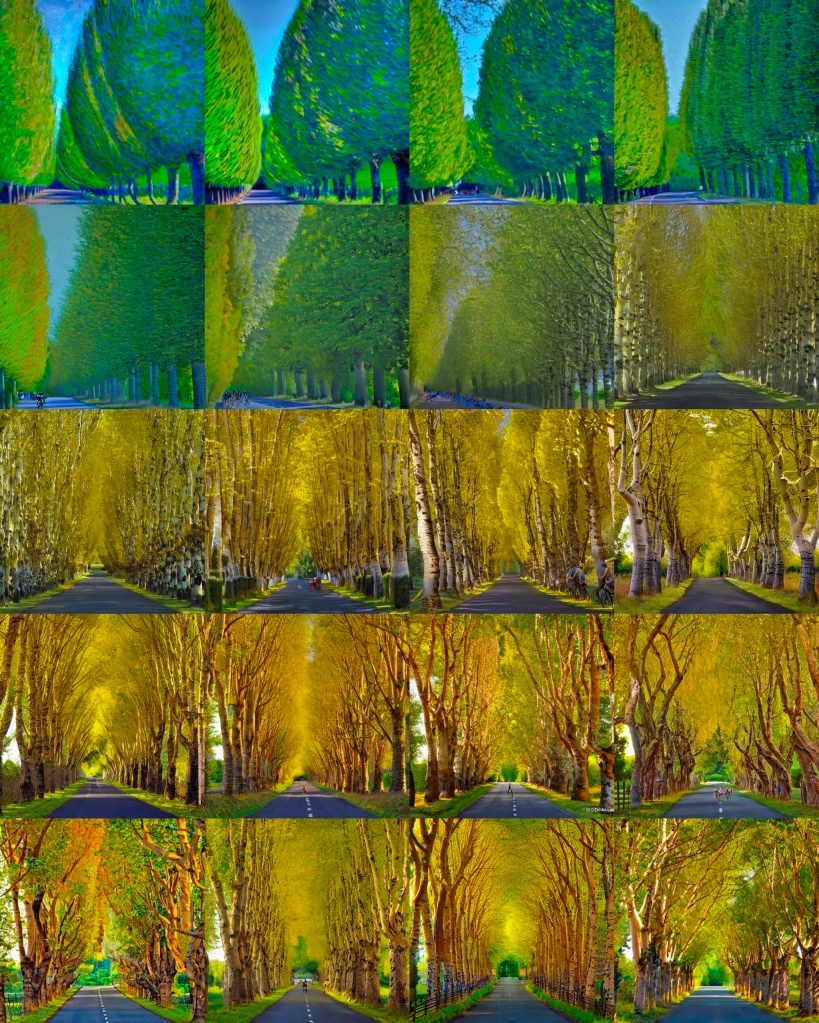
firstimage
Four laps of Richmond Park

When you upload a ride, Strava draws a map using the longitude and latitude coordinates recorded by your GPS device. This article explores ways in which these numbers, along with other metrics, can be used to create interesting images that might have some artistic merit.

The idea was motivated by the huge advances made in the field of Deep Learning, particularly applications for image recognition. However, since datasets come in all shapes and forms, researchers have explored ways of converting different types of data into images.  In a paper published in 2015, the authors achieved success in identifying standard time series by converting them into images.

GPS bike computers typically record snapshots of information every second. What kind of images could these time series generate? It turns out that there are several ways to convert a time series into an image.

Spectrogram

Creating a spectrogram is a standard approach from signal processing that is particularly useful for analysing acoustic files. The spectrogram is a heat map that shows how the underlying frequencies contributing to the signal change over time. Technically, it is derived by calculating the discrete Fourier transform of a window that slides across the time series. I applied this to my regular Saturday morning club ride of four laps around Richmond Park. The image changes a bit once the ride gets going after about 1200 seconds (20 minutes), but, frankly, the result was not particularly illuminating. There is no obvious reason to consider cycling power data as a superposition of frequencies.

spectrogram

Ah! Now we are getting somewhere

The authors of the referenced paper took a different approach to produce things called Gramian Angular Summation Field (GASF), Gramian Angular Difference Field (GADF), and Markov Transition Field (MTF). Read the paper if want to know the details. I created these and something call a Recurrence Plot. All of these methods generate a matrix, by combining every element in the time series with every other element. The underling observations occurring at times t_{1} and t_{2} determine the colour of the pixel at position (t_{1}, t_{2}). Images are symmetric along the lower-left to upper-right diagonal, apart from GADF, which is antisymmetric.

Let’s see how do they look for on four laps of Richmond Park. We have six time series, with corresponding sets of images below. The segmentation of the images is due to periodicity of the data. This is particularly clear in the geographic data (longitude, latitude and altitude). The higher intensity of the main part of the ride is most obvious in the heart rate data. The MTF plots are quite interesting. Scroll down through the images to the next section

data1
Raw time series of power, heart rate, cadence, longitude, latitude and altitude

gasf
Gramian Angular Sum Field

gadf
Gramian Angular Difference Field

mtf
Markov Transition Field

rp
Recurrence Plot

From cycle ride to art

It is one thing to create an image of each item, but how can we combine these to summarise a ride in a single image. I considered two methods of combining time series into a single image: a) create a new image where the vertical and horizontal axes represent different series and b) create a new image by simply adding the corresponding values from two underlying images.

One problem is that some cyclists don’t have gadgets like heart rate monitors and power meters, so I initially restricted myself to just the longitude, latitude and altitude data. Nevertheless, as noted in an earlier blog, it is possible to work out speed, because the time interval is one second between each reading. Furthermore, one can estimate power, from the speed and changes in elevation.

Another problem is that rides differ in length. For this I split the ride into, say, 128 intervals and took the last observation in each interval. So for a 3 hour ride, I’d be sampling about once every 84 seconds.

The chart at the top of this blog was created by first normalising each series to a standard range (-1, +1). Method a) was used to create two images: longitude was added to latitude and altitude was multiplied by speed. These were added using method b). Using these measures will produce pretty much the same chart each time the ride is done. In contrast, an image that is totally unique to the ride can be produced using data relating to the individual rider. The image below uses the same recipe to combine speed, heart rate, power and cadence. If this had been a particularly special ride, the image would be a nice personal memento.

lastimage
A different take on four laps of Richmond Park

For anyone interested in the underlying code, I have posted a Jupyter notebook here.

References

Encoding Time Series as Images for Visual Inspection and Classification Using Tiled Convolutional Neural Networks, Wang Z Oates T, https://www.aaai.org/ocs/index.php/WS/AAAIW15/paper/viewFile/10179/10251