Dreaming of the Giro

fast.ai’s latest version of Practical Deep Learning for Coders Part 2 kicks off with a review of Stable Diffusion. This is a deep neural network architecture developed by Stability AI that is able to convert text into images. With a bit of tweaking it can do all sorts of other things. Inspired by the amazing videos created by Softology, I set out to generate a dreamlike video based on the idea of riding my bicycle around a stage of the Giro d’Italia.

Text to image

As mentioned in a previous post, Hugging Face is a fantastic resource for open source models. I worked with one of fast.ai’s notebooks using a free GPU on Google Colab. In the first step I set up a text-t0-image pipeline using a pre-trained version of stable-diffusion-v1-4. The prompt “a treelined avenue, poplars, summer day, france” generated the following images, where model was more strongly guided by the prompt in each row. I liked the first image in the second row, so I decided to make this the first frame in an initial test video.
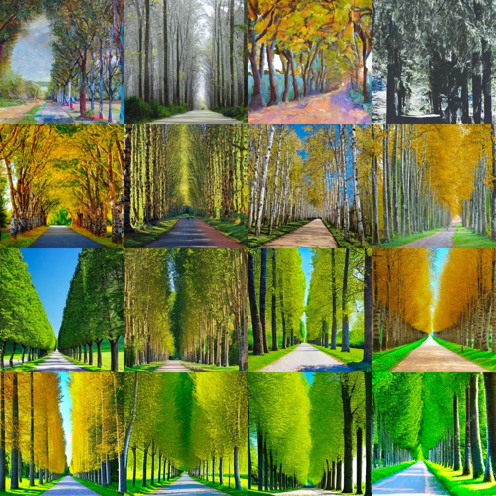
Stable diffusion is trained in a multimodal fashion, by aligning text embeddings with the encoded versions corresponding images. Starting with random noise, the pixels are progressively modified in order to move the encoding of the noisy image closer to something that matches the embedding of the text prompt.

Zooming in

The next step was to simulate the idea of moving forward along the road. I did this by writing a simple two-line function, using fast.ai tools, that cropped a small border off the edge of the image and then scaled it back up to the original size. In order to generate my movie, rather that starting with random noise, I wanted to use my zoomed-in image as the starting point for generating the next image. For this I needed to load up an image-to-image pipeline.

I spent about an hour experimenting with with four parameters. Zooming in by trimming only a couple of pixels around the edge created smoother transitions. Reducing the strength of additional noise enhanced the sense of continuity by ensuring that that subsequent images did not change too dramatically. A guidance scale of 7 forced the model to keep following prompt and not simply zoom into the middle of the image. The number of inference steps provided a trade-off between image quality and run time.

When I was happy, I generated a sequence of 256 images, which took about 20 minutes, and saved them as a GIF. This produced a pleasing, constantly changing effect with an impressionist style.

Back to where you started

In order to make the GIF loop smoothly, it was desirable to find a way to return to the starting image as part of the continuous zooming in process. At first it seemed that this might be possible by reversing the existing sequence of images and then generating a new sequence of images using each image in the reversed list as the next starting point. However, this did not work, because it gave the impression of moving backwards, rather than progressing forward along the road.

After thinking about the way stable diffusion works, it became apparent that I could return to the initial image by mixing it with the current image before taking the next step. By progressively increasing the mixing weight of the initial image, the generated images became closer to target over a desired number of steps as shown below.
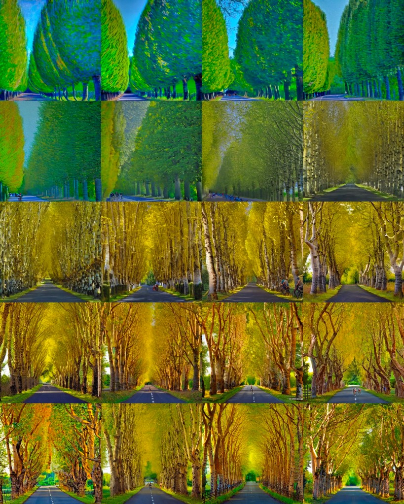
Putting it al together produced the following video, which successfully loops back to its starting point. It is not a perfect animation, because the it zooms into the centre, whereas the vanishing point is below the centre of the image. This means we end up looking up at the trees at some points. But overall it had the effect I was after.
A stage of the Giro

Once all this was working, it was relatively straightforward to create a video that tells a story. I made a list of prompts describing the changing countryside of an imaginary stage of the Giro d’Italia, specifying the number of frames for each sequence. I chose the following.

[‘a wide street in a rural town in Tuscany, springtime’, 25],

[‘a road in the countryside, in Tuscany, springtime’,25],

[“a road by the sea, trees on the right, sunny day, Italy”,50],

[‘a road going up a mountain, Dolomites, sunny day’,50],

[‘a road descending a mountain, Dolomites, Italy’,25],

[‘a road in the countryside, cypress trees, Tuscany’,50],

[‘a narrow road through a medieval town in Tuscany, sunny day’,50]

These prompts produced the video shown at the top of this post. The springtime blossom in the starting town was very effective and the endless climb up into the sunlit Dolomites looked great. For some reason the seaside prompt did not work, so the sequence became temporarily stuck with red blobs. Running it again would make something different. Changing the prompts offered endless possibilities.

The code to run this appears on my GitHub page. If you have a Google account, you can open it directly in Colab and set the RunTime to GPU. You also need a free Hugging Face account to load the stable diffusion pipelines.

Hugging Face

I have been blown away exploring Hugging Face. It’s a community on a mission “to democratize good machine learning”. It provides access to a huge library of state-of-the-art models. So far I have only scratched the surface of what is available, but this blog gives a sample of things I have tried.

At the time of writing, there were 128,463 pre-trained models covering a huge range of capabilities, including computer vision, natural language processing, audio, tabular, multimodal and reinforcement models. The site is set up to make it incredibly easy to experiment with a demo, download a model, run it in a Jupyter notebook, fine-tune it for a specific task and then add it to the space of machine learning apps created by the community. For example, an earlier blog describes my FilmStars app.

Computer vision with text

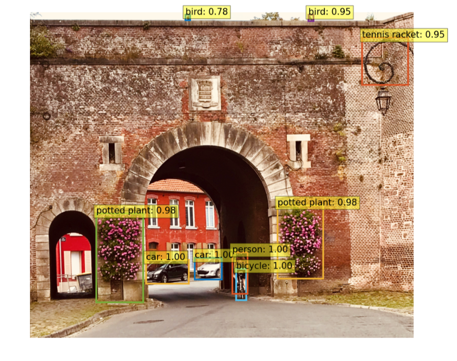
This is an example from an app that uses the facebook/detr-resnet-50 model to identify objects in an image. It successfully located eight objects with high confidence (indicated by the numbers), but it was fooled into thinking part of the curved lamppost in front of the brickwork pattern was a tennis racket (you can see why).

Image-to-text models go further by creating captions describing what is in the image. I used an interactive demo to obtain suggested captions from a range of state-of-the-art models. The best result was produced by the GIT-large model, whereas a couple of models perceived a clocktower .

These models can also answer questions about images. Although all of the answers were reasonable, GIT-large produced the best response when I asked “Where is the cyclist?”

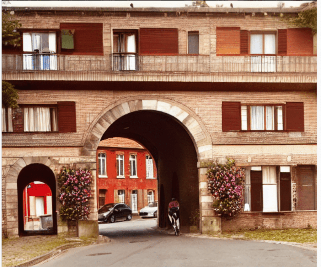
The next image is an example of text-based inpainting with CLIPSeg x Stable Diffusion, where I requested that wall should be replaced with an apartment block. The model successfully generated a new image while preserving the cyclist, flowers, arch, background and even the birds on the roof. I had great fun with this app, imagining what my friend’s house will look like, when it eventually emerges from a building site.

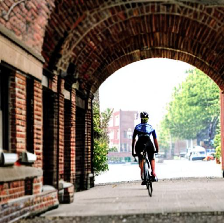
Continuing with the theme of image generation, I reversed the image to caption problem, by asking a stable-diffusion-v1-5 model to generate an image from the caption “a cyclist rides away through an old brick archway in a city”. It came up with an image remarkably similar to what we started with, even including a female cyclist.

Do it yourself

HuggingFace provides various ways for you to download any of the models from its library. The easiest way to do this is to set up a free account on kaggle, which offers a Jupyter notebook environment with access to a GPU.

Using a HuggingFace pipeline, you can run a model with three lines of Python code! Pipelines can be set up for the image models above, but this is an example of the code required to run a text-based natural language processing task. It creates and runs a pipeline that summarises text, using a model specifically trained to generate output in the style of SparkNotes.

from transformers import pipeline
summarizer = pipeline("summarization",model="pszemraj/long-t5-tglobal-base-16384-book-summary")
summarizer("""Sample text from a book...""")

This rather morbid sample text produced the output from Python that follows.

The fact that Henry Armstrong was buried did not seem to him to prove that he was dead: he had always been a hard man to convince. That he really was buried, the testimony of his senses compelled him to admit. His posture — flat upon his back, with his hands crossed upon his stomach and tied with something that he easily broke without profitably altering the situation — the strict confinement of his entire person, the black darkness and profound silence, made a body of evidence impossible to controvert and he accepted it without cavil.

But dead — no; he was only very, very ill. He had, withal, the invalid’s apathy and did not greatly concern himself about the uncommon fate that had been allotted to him. No philosopher was he — just a plain, commonplace person gifted, for the time being, with a pathological indifference: the organ that he feared consequences with was torpid. So, with no particular apprehension for his immediate future, he fell asleep and all was peace with Henry Armstrong.

But something was going on overhead. It was a dark summer night, shot through with infrequent shimmers of lightning silently firing a cloud lying low in the west and portending a storm. These brief, stammering illuminations brought out with ghastly distinctness the monuments and headstones of the cemetery and seemed to set them dancing. It was not a night in which any credible witness was likely to be straying about a cemetery, so the three men who were there, digging into the grave of Henry Armstrong, felt reasonably secure.

From One Summer Night by Ambrose Bierce
[{'summary_text': "Henry's body is buried in the cemetery, but it does not seem to make him any more certain that he is dead. Instead, he seems to be completely ill."}]

Having come this far, it takes only a few steps to fine tune the model to match your desired task, put it into a GitHub repository and launch your own app as a fully fledged member of the Hugging Face community. A nice explanation is available at fast.ai lesson 4.

Predicting the World Champion

A couple of years ago I built a model to evaluate how Froome and Dumoulin would have matched up, if they had not avoided racing against each other over the 2017 season. As we approach the 2019 World Championships Road Race in Yorkshire, I have adopted a more sophisticated approach to try to predict the winner of the men’s race. The smart money could be going on Sam Bennett.

Deep learning

With only two races outstanding, most of this year’s UCI world tour results are available. I decided to broaden the data set with 2.HC classification European Tour races, such as the OVO Energy Tour of Britain. In order to help with prediction, I included each rider’s weight and height, as well as some meta-data about each race, such as date, distance, average speed, parcours and type (stage, one-day, GC, etc.).

The key question was what exactly are you trying to predict? The UCI allocates points for race results, using a non-linear scale. For example, Mathieu Van Der Poel was awarded 500 points for winning Amstel Gold, while Simon Clarke won 400 for coming second and Jakob Fuglsang picked up 325 for third place, continuing down to 3 points for coming 60th. I created a target variable called PosX, defined as a negative exponential of the rider’s position in any race, equating to 1.000 for a win, 0.834 for second, 0.695 for third, decaying down to 0.032 for 20th. This has a similar profile to the points scheme, emphasising the top positions, and handles races with different numbers of riders.

A random forest would be a typical choice of model for this kind of data set, which included a mixture of continuous and categorical variables. However, I opted for a neural network, using embeddings to encode the categorical variables, with two hidden layers of 200 and 100 activations. This was very straightforward using the fast.ai library. Training was completed in a handful of seconds on my MacBook Pro, without needing a GPU.

After some experimentation on a subset of the data, it was clear that the model was coming up with good predictions on the validation set and the out-of-sample test set. With a bit more coding, I set up a procedure to load a start list and the meta-data for a future race, in order to predict the result.

Predictions

With the final start list for the World Championships Road Race looking reasonably complete, I was able to generate the predicted top 10. The parcours obviously has an important bearing on who wins a race. With around 3600m of climbing, the course was clearly hilly, though not mountainous. Although the finish was slightly uphill, it was not ridiculously steep, so I decided to classify the parcours as rolling with a flat finish

PositionRiderPrediction
1Mathieu Van Der Poel0.602
2Alexander Kristoff0.566
3Sam Bennett0.553
4Peter Sagan0.540
5Edvald Boasson Hagen0.507
6Greg Van Avermaet0.500
7Matteo Trentin0.434
8Michael Matthews0.423
9Julian Alaphilippe0.369
10Mike Teunissen0.362

It was encouraging to see that the model produced a highly credible list of potential top 10 riders, agreeing with the bookies in rating Mathieu Van Der Poel as the most likely winner. Sagan was ranked slightly below Kristoff and Bennett, who are seen as outsiders by the pundits. The popular choice of Philippe Gilbert did not appear in my top 10 and Alaphilippe was only 9th, in spite of their recent strong performances in the Vuelta and the Tour, respectively. Riders in positions 5 to 10 would all be expected to perform well in the cycling classics, which tend to be long and arduous, like the Yorkshire course.

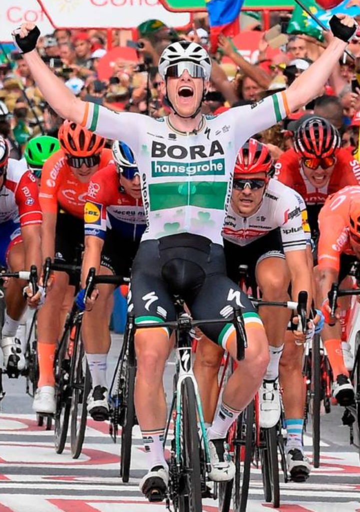
For me, 25/1 odds on Sam Bennett are attractive. He has a strong group of teammates, in Dan Martin, Eddie Dunbar, Connor Dunne, Ryan Mullen and Rory Townsend, who will work hard to keep him with the lead group in the hillier early part of the race. Then he will then face an extremely strong Belgian team that is likely to play the same game that Deceuninck-QuickStep successfully pulled off in stage 17 of the Vuelta, won by Gilbert. But Bennett was born in Belgium and he was clearly the best sprinter out in Spain. He should be able to handle the rises near the finish.

A similar case can be made for Kristoff, while Matthews and Van Avermaet both had recent wins in Canada. Nevertheless it is hard to look past the three-times winner Peter Sagan, though if Van Der Poel launches one of his explosive finishes, there is no one to stop him pulling on the rainbow jersey.

Appendix

After the race, I checked the predicted position of the eventual winner, Mads Pedersen. He was expected to come 74th. Clearly the bad weather played a role in the result, favouring the larger riders, who were able to keep warmer. The Dane clearly proved to be the strongest rider on the day.

References

Code used for this project

Can self-driving cars detect cyclists?

Screenshot 2019-05-10 at 14.05.59

Self-driving cars employ sophisticated software to interpret the world around them. How do these systems work? And how good are they at detecting cyclists? Can cyclists feel safe sharing roads with an increasing number of vehicles that make use of these systems?

How hard is it to spot a cyclist?

Vehicles can use a range of detection systems, including cameras, radar and lidar.  Deep learning techniques have become very good at identifying objects in photographic images. So one important question is how hard is it to spot a cyclist in a photo taken from a moving vehicle?

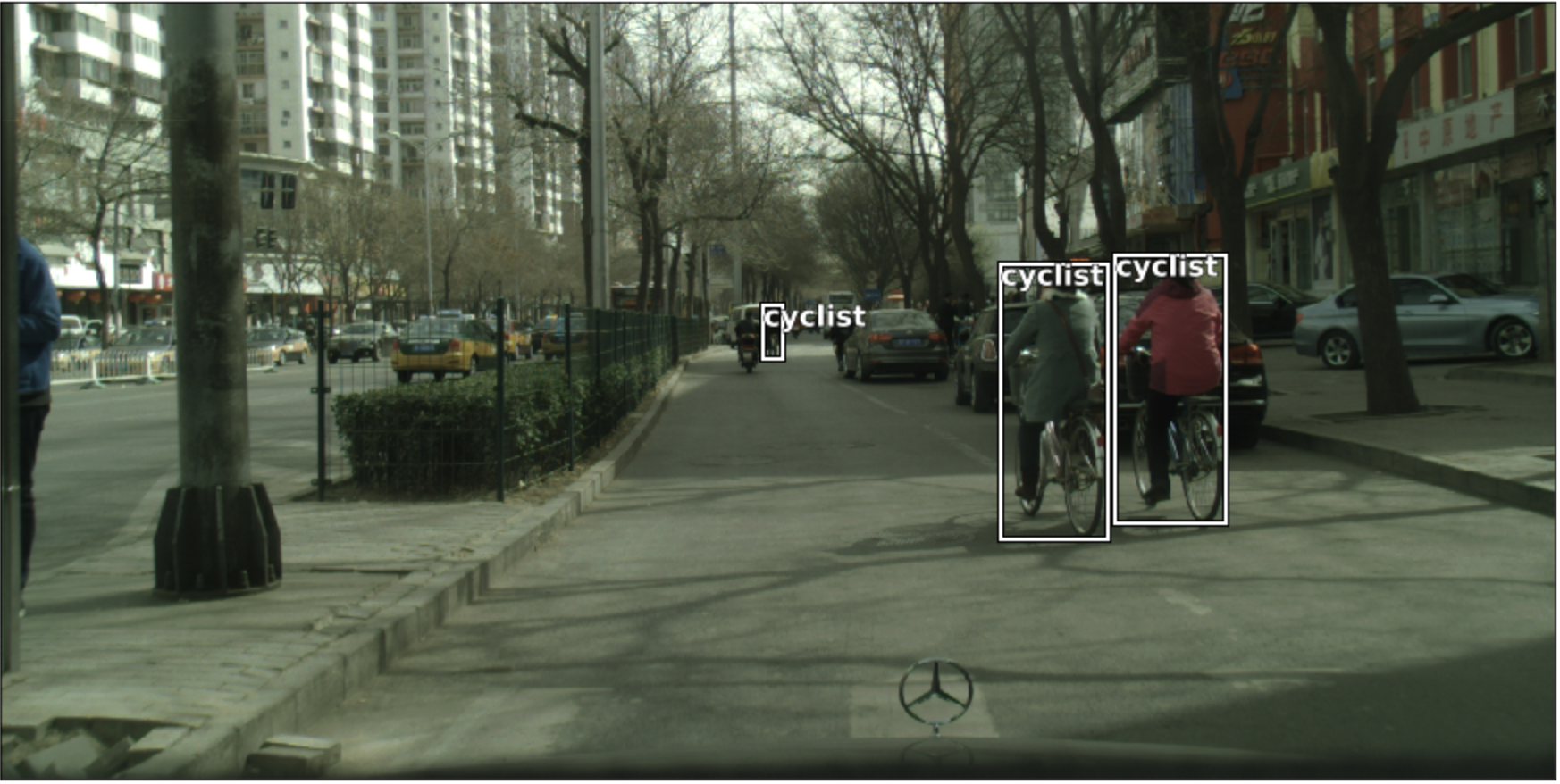
Researchers at Tsinghua University, working in collaboration with Daimler, created a publicly available collection of dashboard camera photos, where humans have painstakingly drawn boxes around other road users. The data set is used by academics to benchmark the performance of their image recognition algorithms. The images are rather grey and murky, reflecting the cloudy and polluted atmosphere of the Chinese city location. It is striking that, in the majority of cases, the cyclists are very small, representing around 900 pixels out of the 2048 x 1024 images, i.e. less than 0.05% of the total area. For example, the cyclist in the middle of the image above is pretty hard to make out, even for a human.

Object-detecting neural networks are typically trained to identify the subject of a photo, which normally takes up are significant portion of the image. Finding a tall, thin segment containing a cyclist is significantly more difficult.

If you think about it, the cyclist taking up the largest percentage of a dash cam image will be riding across the direction of travel, directly in front of the vehicle, at which point it may be too late to take action. So a crucial aspect of any successful algorithm is to find more distant cyclists, before they are too close.

Setting up the problem

Taking advantage of skills acquired on the fast.ai course on deep learning, I decided to have a go at training a neural network to detect cyclists. Many of the images in the Tsinghua Daimler data set include multiple cyclists. In order to make the problem more manageable, I set out to find the single largest cyclist in each image.

If you are not interested in the technical bit, just scroll down to the results.

The technical bit

In order to save space on my drive, I downloaded about a third of the training set. The 3209 images were split 80:20 to create a training and validation sets. I also downloaded 641 unseen images that were excluded from training and used only for testing the final model.

I used transfer learning to fine-tune a neural network using a pre-trained ResNet34 backbone, with a customised head designed to generate four numbers representing the coordinates of a bounding box around the largest object in each image. All images were scaled down to 224 pixel squares, without cropping. Data augmentation added variation to the training images, including small rotations, horizontal flips and adjustments to lighting.

It took a couple of hours to train the network on my MacBook Pro, without needing to resort to a cloud-based GPU, to produce bounding boxes with an average error of just 12 pixels on each coordinate. The network had learned to do a pretty good job at detecting cyclists in the training set.

Results

The key step was to test my neural network on the set of 641 unseen images. The results were impressive: the average error on the bounding box coordinates was just 14 pixels. The network was surprisingly good at detecting cyclists.

oosImages

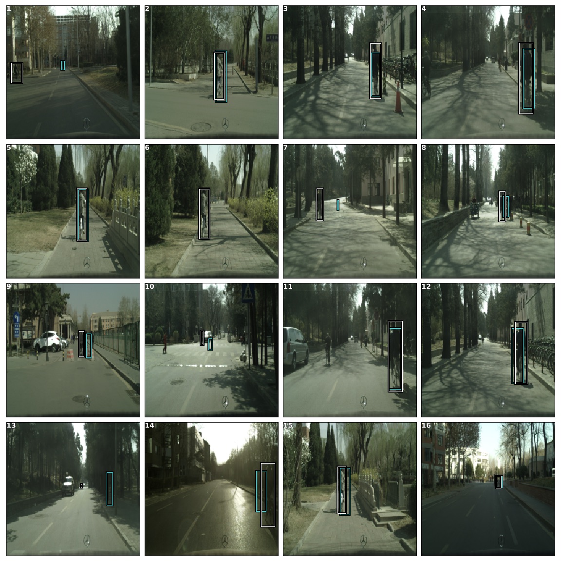
The 16 photos above were taken at random from the test set. The cyan box shows the predicted position of the largest cyclist in the image, while the white box shows the human annotation. There is a high degree of overlap for eleven cyclists 2, 3, 4, 5, 6, 8, 11, 12, 14, 15 and 16. Box 9 was close, falling between two similar sized riders, but 7 was a miss. The algorithm failed on the very distant cyclists in 1, 10 and 13. If you rank the photos, based on the size of the cyclist, we can see that the network had a high success rate for all but the smallest of cyclists.

In conclusion, as long as the cyclists were not too far away, it was surprisingly easy to detect riders pretty reliably, using a neural network trained over an afternoon.  With all the resources available to Google, Uber and the big car manufacturers, we can be sure that much more sophisticated systems have been developed. I did not consider, for example, using a sequence of images to detect motion or combining them with data about the motion of the camera vehicle. Nor did I attempt to distinguish cyclists from other road users, such as pedestrians or motorbikes.

After completing this project, I feel reassured that cyclists of the future will be spotted by self-driving cars. The riders in the data set generally did not wear reflective clothing and did not have rear lights. These basic safety measures make cyclists, particularly commuters, more obvious to all road users, whether human or AI.

Car manufacturers could potentially develop significant goodwill and credibility in their commitment to road safety by offering cyclists lightweight and efficient beacons that would make them more obvious to automated driving systems.

References

“A new benchmark for vision-based cyclist detection”, X. Li, F. Flohr, Y. Yang, H. Xiong, M. Braun, S. Pan, K. Li and D. M. Gavrila, in proceedings of IEEE Intelligent Vehicles Symposium (IV), pages 1028-1033, June 2016

Link to Jupyter notebook

Learning the language of the Giro

Fausto_Coppi

Computers are becoming ever better at natural language processing (NLP). I set up a neural network as a language model and loaded a set of pre-trained weights on my MacBook Pro, to see what it could do. After priming it with some text about the Giro d’Italia, this is what the model produced as a continuation.

Priming text: The Giro d’ Italia (Italian pronunciation: [ˈdʒiːro diˈtaːlja]; English: Tour of Italy; also known as the Giro) is an annual multiple-stage bicycle race primarily held in Italy, while also occasionally passing through nearby countries. The first race was organized in 1909 to increase sales of the newspaper La Gazzetta dello Sport; however it is currently run by RCS Sport. The race has been held annually since its first edition in 1909, except when it was stopped for the two world wars. As the Giro gained prominence and popularity the race was lengthened, and the peloton expanded from primarily Italian participation to riders from all over the world.

Computer generated continuation:  the race was won by the italian rider , giovanni di u_n , who won the race in the first leg of the race . the race was won by italian rider giovanni u_n , who won the race by a margin of two lengths .
= = = world tour = = =
the tour de france was the first of the tour de france . the tour de france was won by the reigning world champion , the reigning world champion , who had won the tour de france in the previous year ‘s race …

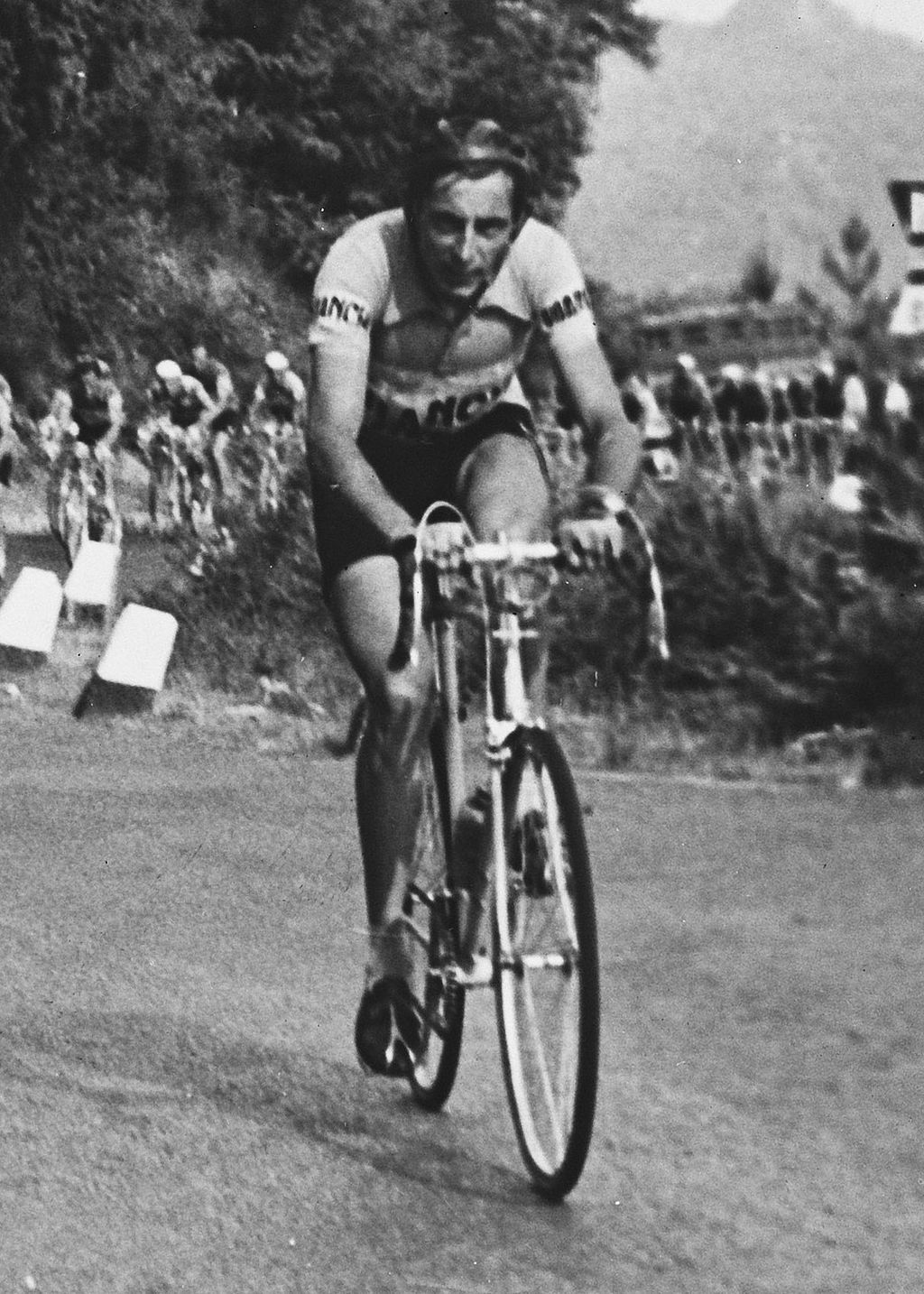
The output may not make a lot of sense, but the point is that it looks like English (in lower case). The grammar is reasonable, with commas, fullstops and a header inserted in  a logical way. Furthermore, the model has demonstrated some understanding of the context by suggesting that the Giro could be won by an Italian ride called Giovanni. The word “u_n” stands for unknown, which is consistent with the idea that an Italian surname may not be a familiar English word. It turns out that a certain Giovanni Di Santi raced against Fausto Coppi (pictured above) in the 1940 Giro, though he did not win the first stage. In addition to this, the model somehow knew that the Giro, in common with the Tour the France, is a World Tour event that could be won by the reigning world champion.

I found this totally amazing. And it was not a one off: further examples on random topics are included below. This neural network is just an architecture, defining a collection of matrix multiplications and transformations, along with a set of connection weights. Admittedly there are a lot of connection weights: 115.6 million of them, but they are just numbers. It was not explicitly provided with any rules about English grammar or any domain knowledge.

How could this possibly work?

In machine learning, language models are assessed on a simple metric: accuracy in predicting the next word of a sentence. The neural network approach has proved to be remarkably successful. Given enough data and a suitable architecture, deep learning now far outstrips traditional methods that relied on linguistic expertise to parse sentences and apply grammatical rules that differ across languages.

I was experimenting with an AWD-LSTM model originally created by Stephen Merity. This is a recurrent neural network (RNN) with three LSTM layers that include dropout. The pre-trained weights for the wt103 model were generated by Jeremy Howard of fast.ai, using a large corpus of text from Wikipedia.

Jeremy Howard converted the Wikipedia text into tokens. A tokeniser, such as spaCy,  breaks text into words and punctuation, resulting in a vocabulary of tokens that are indexed as integers. This allows blocks of text to be fed into the neural network as lists of numbers. The outputs are numbers that can be converted back into the predicted words.

The wt103 model includes a linear encoder that creates embeddings of word tokens. These are passed through three LSTM layers whose states are able to retain a memory of previous words or context. The result is passed through a decoder, employing the same weights as the encoder, to produce a softmax output that can be treated as a set of probabilities, across the vocabulary, to predict the next word token. Special forms of dropout were employed, as described in the paper, to limit overfitting and make the model more robust.

The network was trained by minimising cross-entropy loss using stochastic gradient descent. A technique called back propagation through time (BPTT) introduced some random variation into the length of the blocks of text employed in each training batch. The connection weights were iteratively improved towards optimal values.

OK, but so what?

Impressive as it may be for a neural network to spout highly plausible but nonsensical English, what possible use could this have? Well, suppose you want to automate the separation of texts into different categories, for example, distinguish different authors or determine the sentiment of tweets or predict the reaction of the stock market to news items or identify the sentiment of movie reviews. Fine-tuning a neural network that already has a good knowledge of English provides a huge advantage over starting from scratch. In lesson 10 of the fast.ai course, Jeremy Howard demonstrates how this approach can be used to achieve state of the art results on the widely used IMDB movie review data set.

Further examples

In the first example, the network finishes the sentence about a hurricane in perfect English.  Next, it comes up with the name of a critic (actually a rock music critic rather than a book reviewer, but heh!) and it makes use of its LSTM to open and close quotation marks. In the bean example, it amazingly starts describing flowers and correctly converts their dimensions from centimetres to inches!

My code can be found here.

Priming text: Hurricane Ivan was a large long Cape Verde hurricane that caused widespread damage in the Caribbean and United States The cyclone was

Computer generated continuation:  the first hurricane to strike the united states since hurricane katrina in 2005 .

Priming text: The book was widely acclaimed by the critics.

Computer generated continuation: the book was published in the united states by the american library association on june 1 , 2006 .

= = = critical response = = =

the book received mixed reviews from critics . the new york times reviewer robert christgau called it ” a great book ” and ” a great book ” . he praised the book ‘s ” strong , strong , and well – written ” prose , and the ” excellent ” prose .

Priming text: Most varieties of bean grow either as an erect bush or as a climbing plant, but a few important kinds are of intermediate form. Dwarf and semiclimbers are grown extensively. When the climbing type is grown for its immature pods, artificial supports are necessary to facilitate harvesting. Varieties differ greatly in size, shape, colour, and fibrousness or tenderness of the immature pods. In general, varieties grown for dry mature seeds produce pods that are too fibrous to be eaten at any state of development. Most edible-podded beans produce relatively low yields of mature seeds, or seeds that are of low eating quality. Seed colours range from white through green, yellow, tan, pink, red, brown, and purple to black in solid colours and countless contrasting patterns. Seed shapes range from nearly spherical to flattened, elongated, and kidney-shaped. Pods are of various shades of green, yellow, red, and purple and splashed with red or purple; pod shapes range from flat to round, smooth to irregular, and straight to sharply curved; length ranges from 75 to 200 millimetres (3 to 8 inches) or more.

Computer generated continuation:  the most common form of the flower is the flower spike , which is a characteristic of the flower spike . the flower is made up of a series of small , cylindrical , cylindrical , cylindrical , cylindrical stems that are up to 10 cm ( 3.9 in ) long and 2.5 cm ( 0.98 in ) wide . the flower spikes are arranged in a series of three or four pairs of flowers 


Cycling Through Artistic Styles

HR

My earlier post on cycling art provided an engaging way to consider the creative potentials of deep learning. I have found myself frequently gravitating back to the idea, using the latest code available over at fast.ai. The method uses a neural network to combine the content of a photograph with the style of an artist, but I have found that it takes a few trials to find the right combination of content versus style. This led to the idea of generating a range of images and then running them together as a movie that gradually shifts between the base image to a raw interpretation of the artist’s style.

Artistic styles

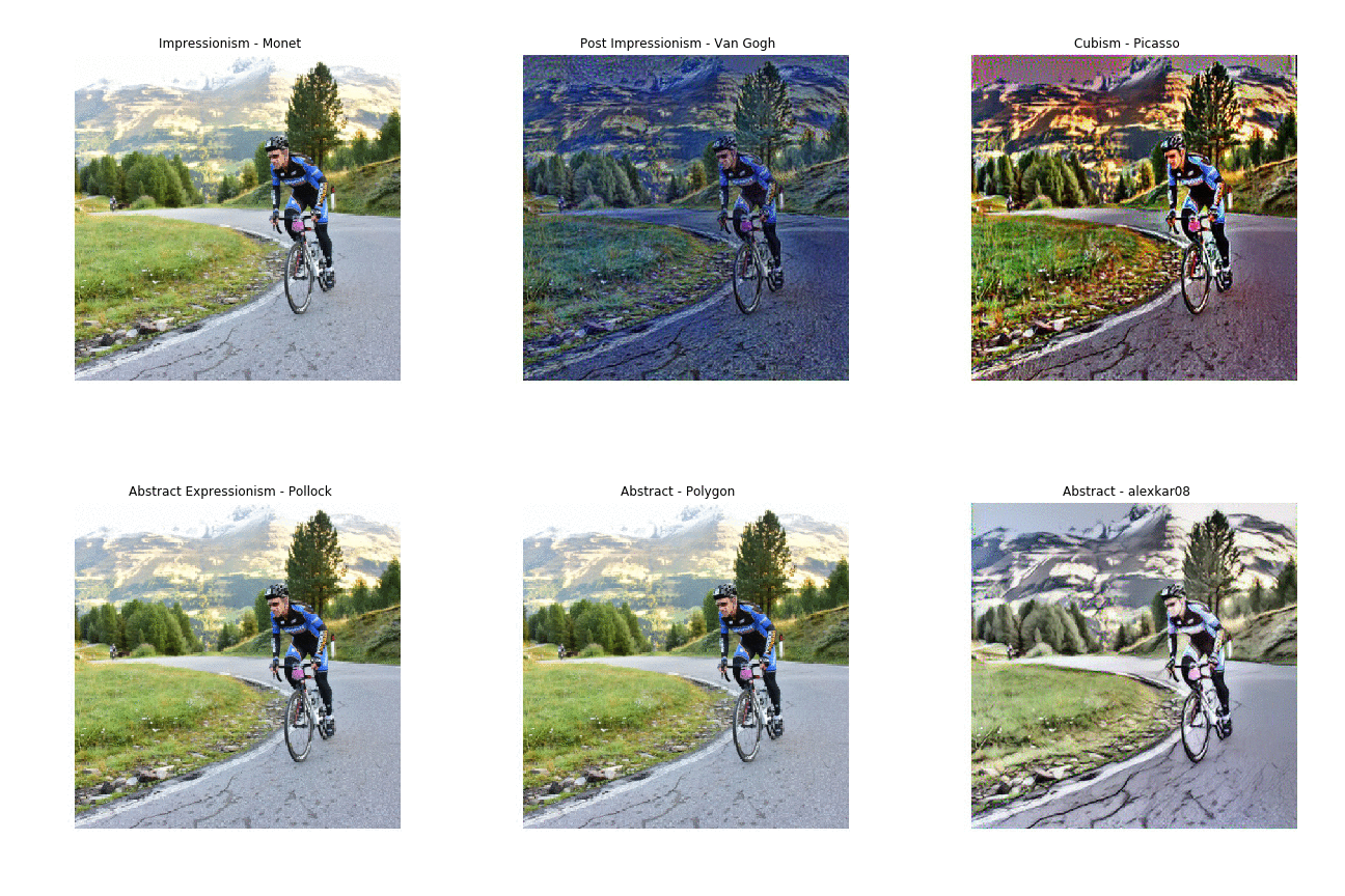
Using a range of artistic styles from impressionist to abstract, the weights that produced the most interesting images varied according to the photograph and artistic style.

My selected best images are shown below, next to snippets of the corresponding artworks. It turned out that the impressionist artists (Monet, Van Gogh, Cézanne and Braque) maintained the content of the image, in spite of being more heavily weighted to artistic style. In contrast, the more monochromatic styles (O’Keeffe, Polygons, Abstract as well as Dali) needed to be more strongly weighted towards content, in order to preserve the cyclist in the image. The selections for Picasso and Pollock were evenly balanced.

Every image is unique and sometimes some real surprises pop up. For example, using Picasso’s style, the mountains are interpreted as rooftops, complete with windows and doors. Strange eyes peer out the background of finger-shapes in the Dali image and the mountains have become Monet’s water lilies. The Pollock image came out very nicely.

Deep learning

The approach was based on the method described in the paper referenced below. Running the code on a cloud-based GPU, it took about 30 seconds for a neural network to learn to generate in image with the desired characteristics. The learning process was achieved by minimising a loss function, using gradient descent. The clever part lay in defining an appropriate loss function. In this instance, the sample image was passed through a separate pre-trained neural network (VGG16), where the activations, at various layers in the network, were compared to those generated by the photograph and the artwork. The loss function combined the difference in photographic content with the difference in artistic style, where the critical parameter was the content weighting factor.

I decided to vary the content weighting factor logarithmically between around 0.1 and 100, to obtain a full range of content to style combinations. A movie was be produced simply by packing together the images one after the other.

References

A Neural Algorithm of Artistic Style, Leon A. Gatys, Alexander S. Ecker, Matthias Bethge


What are you looking at?

Screen Shot 2018-05-06 at 18.48.40.png

In a recent blog, I described an experiment to train a deep neural network to distinguish between photographs of Vincenzo Nibali and Alejandro Valverde, using a very small data set of images. In the conclusion, I suggested that the network was probably basing its decisions more on the colours of the riders’ kit rather than on facial recognition. This article investigates what the network was actually “looking at”, in order to understand better how it was making decisions.

The issues of accountability and bias were among the topics discussed at the last NIPS conference. As machine learning algorithms are adopted across industry, it is important for companies to be able to explain how conclusions are reached. In many instances, it is not acceptable simply to rely on an impenetrable black box. AI researchers and developers need to be able to explain what is going on inside their models, in order to justify decisions taken. In doing so, some worrying instances of bias have been revealed in the selection of data used to train the algorithms.

I went back to my rider recognition model and used an approach called “Class Activation Maps” to identify which parts of the images accounted for the network’s choice of rider. Making use of the code provided in lesson 7 of the course offered by fast.ai, I took advantage of my existing small set of training, validation and test images of the two famous cyclists. Starting with a pre-trained version of ResNet34, the idea was to replace the last two layers with four new ones, the crucial one being a convolutional layer with two outputs, matching the number of cyclists in the classification task. The two outputs of this layer were 7×7 matrix representations of the relevant image.

The final predictions of the model came from a softmax of a flattened average pooling of these 7×7 representations. The softmax output gave the probabilities of Nibali and Valverde respectively. Since there was no learning beyond the final convolution, the activations of the two 7×7 matrices represented the “Nibali-ness” and “Valverde-ness” of the image. This could be displayed as a heat map on top of the image.

Examples are shown below for the validation set of 10 images of Nibali followed by 10 of Valverde. The yellow patch of the heat map highlights the part of the image that led to the prediction displayed above each image. Nine out of ten were correct for Nibali and six for Valverde.

Screen Shot 2018-05-06 at 18.10.00.png
Class Activation Maps applied to the validation set

The heat maps were very helpful in understanding the model’s decision making process. It seemed that for Nibali, his face and helmet were important, with some attention paid to the upper part of his blue Astana kit. In contrast, the network did a very good job at identifying the M on Valverde’s Moviestar kit. It was interesting to note that the network succeeded in spotting that Nibali was wearing a Specialized helmet whereas Valverde had a Catlike design. Three errors arose in the photos of his face, which was mistaken for Nibali’s. In fact, any picture of a face led to a prediction of Nibali, as demonstrated by the cropped image below that was used for training.

Screen Shot 2018-05-06 at 18.21.58

Why should that be? Looking back at the training set, it turned out that, by chance, there were far more mugshots of Nibali, while there were more photos of Valverde riding his bike, with his face obscured by sunglasses. This was an example of unintentional bias in the training data, providing a very useful lesson.

The final set of pictures shows the predictions made on the out-of-sample test set. All the predictions are correct, except the first one, where the model failed to spot the green M on Valverde’s chest and mistook the blurred background for Nibali. Otherwise the results confirmed that the network looked at Nibali’s face, the rider’s helmet or Valverde’s kit. It also remembered seeing an image of Nibali holding the Giro trophy in the training set.

Screen Shot 2018-05-06 at 18.34.38.png
Class Activation Maps applied to the test set

In conclusion, Class Activation Maps provide a useful way of visualising the activations of hidden laters in a deep neural network. This can go some way to accounting for the decisions that appear in the output. The approach can also help identify unintentional bias in the training set.

Which team is that?

Screen Shot 2018-04-11 at 11.18.09

My last blog explored the effectiveness of deep learning in spotting the difference between Vincenzo Nibali and Alejandro Valverde. Since the faces of the riders were obscured in many of the photos, it is likely that the neural network was basing its evaluations largely on the colours of their team kit. A natural next challenge is to identify a rider’s team from a photograph. This task parallels the approach to the kaggle dog breed competition used in lesson 2 of the fast.ai course on deep learning.

Eighteen World Tour teams are competing this year. So the first step was to trawl the Internet for images, ideally of riders in this year’s kit. As before, I used an automated downloader, but this posed a number of problems. For example, searching for “Astana” brings up photographs of the capital of Kazakhstan. So I narrowed things down by searching for  “Astana 2018 cycling team”. After eliminating very small images, I ended up with a total of about 9,700 images, but these still included a certain amount of junk that I did have the time to weed out, such as photos of footballers or motorcycles in the “Sky Racing Team”,.

The following small sample of training images is generally OK, though it includes images of Scott bikes rather than Mitchelton-Scott riders and  a picture of  Sunweb’s Wilco Kelderman labelled as FDJ. However, with around 500-700 images of each team, I pressed on, noting that, for some reason, there were only 166 of Moviestar and these included the old style kit.

Screen Shot 2018-04-11 at 10.18.54.png
Small sample of training images

For training on this multiple classification problem, I adopted a slightly more sophisticated approach than before. Taking a pre-trained Resnet50 model, I performed some initial fine-tuning, on images rescaled to 224×224. I settled on an optimal learning rate of 1e-3 for the final layer, while allowing some training of lower layers at much lower rates. With a view to improving generalisation, I opted to augment the training set with random changes, such as small shifts in four directions, zooming in up to 10%, adjusting lighting and left-right flips. After initial training, accuracy was 52.6% on the validation set. This was encouraging, given that random guesses would have achieved a rate of 1 in 18 or 5.6%.

Taking a pro tip from fast.ai, training proceeded with the images at a higher resolution of 299×299. The idea is to prevent overfitting during the early stages, but to improve the model later on by providing more data for each image. This raised the accuracy to 58.3% on the validation set. This figure was obtained using a trick called “test time augmentation”, where each final prediction is based on the average prediction of five different “augmented” versions of the image in question.

Given the noisy nature of some of the images used for training, I was pleased with this result, but the acid test was to evaluate performance on unseen images. So I created a test set of two images of a lead rider from each squad and asked the model to identify the team. These are the results.

75 percent right.png
75% accuracy on the test set

The trained Resnet50 correctly identified the teams of 27 out of 36 images. Interestingly, there were no predictions of MovieStar or Sky. This could be partly due to the underrepresentation of MovieStar in the training set. Froome was mistaken for AG2R and Astana, in column 7, rows 2 and 3. In the first image, his 2018 Sky kit was quite similar to Bardet’s to the left and in the second image the sky did appear to be Astana blue! It is not entirely obvious why Nibali was mistaken for Sunweb and Astana, in the top and bottom rows. However, the huge majority of predictions were correct. An overall  success rate of 75% based on an afternoon’s work was pretty amazing.

The results could certainly be improved by cleaning up the training data, but this raises an intriguing question about the efficacy of artificial intelligence. Taking a step back, I used Bing’s algorithms to find images of cycling teams in order to train an algorithm to identify cycling teams. In effect, I was training my network to reverse-engineer Bing’s search algorithm, rather than my actual objective of identifying cycling teams. If an Internet search for FDJ pulls up an image of Wilco Kelderman, my network would be inclined to suggest that he rides for the French team.

In conclusion, for this particular approach to reach or exceed human performance, expert human input is required to provide a reliable training set. This is why this experiment achieved 75%, whereas the top submissions on the dog breeds leaderboard show near perfect performance.

Valverde or Nibali?

Alejandro Valverde has kicked off the 2018 season with an impressive series of wins. Meanwhile Vincenzo Nibali delighted the tifosi with his victory in Milan San Remo. It is pretty easy to tell these two riders apart in the pictures above, but could computer distinguish between them?

Following up on my earlier blogs about neural networks, I have been taking a look at the updated version of fast.ai’s course on deep learning. With the field advancing at a rapid pace, this provides a good way to staying up to date with the state of the art. For example, there are now a couple of cheaper alternatives to AWS for accessing high powered GPUs, offered by Paperspace and Crestle. The latest fast.ai libraries include many new tools that work extremely well in practice.

There’s a view that deep learning requires hours of training on high-powered supercomputers, using thousands (or millions) of labelled examples, in order to learn to perform computer vision tasks. However, newer architectures, such as ResNet, are able to run on much smaller data sets. In order to test this, I used an image downloader to grab photos of Nibali and Valverde and manually selected about 55 decent pictures of each one.

I divided the images into a training set with about 40 images of each rider, a validation set with 10 of each and a test set containing the rest. Nibali appears in a range of different coloured jerseys, though the Astana blue is often present. Valverde is mainly wearing the old dark blue Movistar kit with a green M. There were more close-up shots of Nibali’s face than Valverde.

Screen Shot 2018-04-03 at 18.30.08.png

I was able to fine-tune a pre-trained ResNet neural network to this task, using some of the techniques from the fast.ai tool box, each designed to improve generalisation. The first trick was to augment the training set by performing minor transformations of the images at random, such as taking a mirror image, shifting left or right and zooming in a bit. The second set of tricks varied the rate of learning as the algorithm iterated repeatedly through the training set. A final useful technique created a set of variants of each test image and took the average of the predictions. Everything ran at lightning speed on a Paperspace GPU. After a run time of just a few minutes, the ResNet was able to  score 17 out of 20 on the following validation set.

Screen Shot 2018-04-03 at 18.49.27.png

The confusion matrix shows that the model correctly identified all the Nibali images, but it was wrong on three pictures of Valverde. The first incorrect image (below) shows Valverde in the red leader’s jersey of the Tour of Murcia, which is not dissimilar to Nibali’s new Bahrain Merida kit, though he was wearing red in two of his training images. In the second instance, the network was fooled by the change in colour of Moviestar’s kit, which had become rather similar to Astana’s light blue. The figure of 0.41 above the close-up image indicates that the model assigned only a 41% probability that the image was Valverde. It probably fell below the critical 50% level, in spite of the blue/green colours, because there were were far more close-up shots of Nibali than Valverde in the training set.

Overall of 17 out of 20 on the validation set is impressive. However, the network had access to the validation set during training, so this result is “in sample”. A proper  “out of sample” evaluation of the model’s ability made use the following ten images, comprising the test set that was kept aside.

Screen Shot 2018-04-03 at 21.21.59

Amazingly, the model correctly identified 9 out of the 10 pictures it had not seen before. The only error was the Valverde selfie shown in the final image. In order to work better in practice, the training set would need to include more examples of the riders’ 2018 kit. A variant of the problem would be to identify the team rather than the rider. The same network can be trained for multiple classes rather than just two.

This experiment shows that it is pretty straightforward to run state of the art image recognition tools remotely on a GPU somewhere in the cloud and come up with pretty impressive results, even with a small data set.

The next blog describes how to identify a rider’s team.


Deep Learning – Faking It

Screen Shot 2017-08-20 at 15.01.01
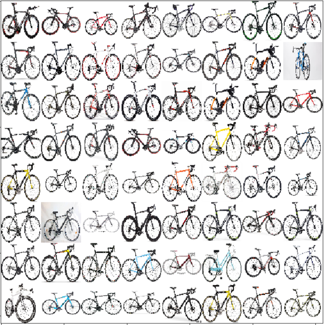
Thumbnails of real bikes (Bianchi, Giant, Cube…)

Screen Shot 2017-08-20 at 15.01.15
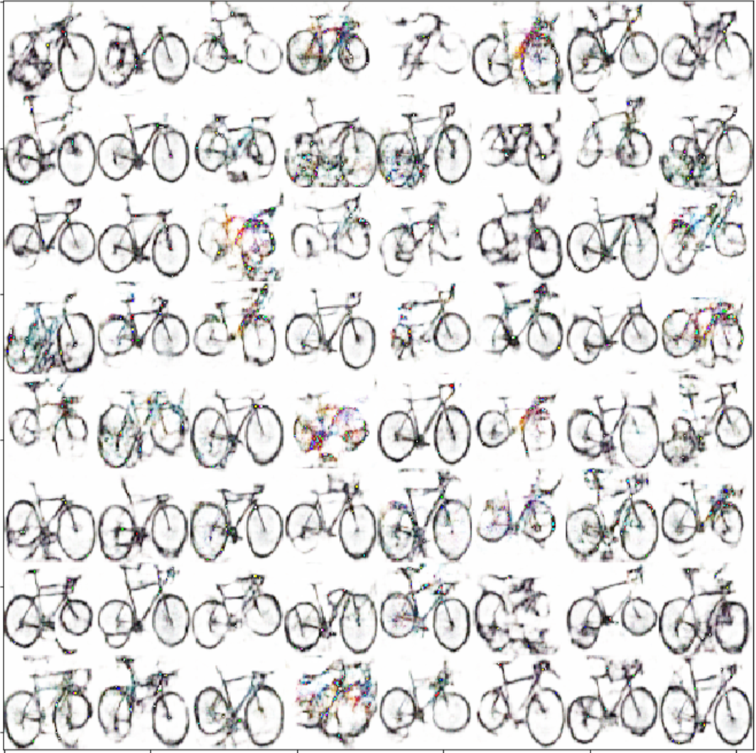
Fake thumbnails generated randomly by Wasserstein Generative Adversarial Network

My last blog showed the results of using a deep convolutional neural network to apply different artistic styles to a photograph of cyclist.  This article looks at the trendy topic of Generative Adversarial Networks (GANs). Specifically, I investigate the application of a Wasserstein GAN to generate thumbnail images of bicycles.

In the field of machine learning, a generative model is a model designed to produce examples from a particular target distribution. In statistics, the output might be samples from a Gaussian distribution, but we can extend the idea to create a model that produces examples of sonnets in the style of Shakespeare or pictures of cats… or bicycles.

The adversarial framework introduces an attractive idea from game theory: to create a competitive form of learning. While a generator learns from a corpus of real examples how to create realistic “fakes”, a discriminator (or critic) learns to distinguish been fakes and authentic examples. In fact, the generator is given the objective of trying to fool the discriminator. As the discriminator improves, the generator is driven to enhance the authenticity of its output. This creates a virtuous cycle.

When originally proposed in 2014, Generative Adversarial Networks stimulated much interest, but it proved hard to make them work reliably in practice. One problem was “mode collapse”, where the generator becomes stuck, producing the same output all the time. However, this changed with the publication of a recent paper, explaining how earlier problems could be overcome by using a so-called Wasserstein loss function.

As an experiment, I downloaded a batch of images of bicycles from the Internet. After manually removing pictures with riders and close-ups of components, there were about 1,200 side views of road bikes (mostly with handlebars to the right, so you can see the chainset). After a few experiments, I reduced the dataset to the 862 images, by automatically selecting bikes against a white background.

Screen Shot 2017-08-20 at 14.45.29
Sample of real bike images

As a participant of part 2 of the excellent fast.ai deep learning course, I made use of WGAN code that runs using Pytorch. I loaded the bike images at thumbnail size of 64×64 (training with larger images exceeded the memory constraints of the p2.large GPU I’m running on AWS). It was initially disappointing to experience the mode collapse problem, especially because the authors of the WGAN paper claimed never to have encountered it. However, speeding up the learning rate of the generator seemed to solve the problem.

Although each fake was created from a completely random starting point, the generator learned to produce images against a white background, with two circles joined by lines. After a couple of hundred iterations the WGAN began to generate some recognisably bicycle-like images. Notice the huge variety. Some of the best ones are shown at the top of this post.

Screen Shot 2017-08-20 at 14.41.19
Sample of images generated by WGAN

I tried to improve the WGAN’s images, using another deep learning tool: super resolution. This amazing technique is used to solve the seemingly impossible task of converting images from low resolution to high resolution. It is achieved by taking downgraded versions of a large dataset of high resolution images, then training a neural network to reproduce a high-res version from the corresponding low-res input. A super resolution network is able to learn about certain properties of the world, for example, it converts jagged curves into smooth ones – a feature I’d hoped might be useful for making wheels look rounder.

Example of a super resolution network on real photographs

Unfortunately, my super resolution experiments did not lead to the improvement I’d hoped for. Two possible explanations are that a) the fake images were not low-res photos and b) the network had been trained on many types of images other than bicycles with white backgrounds.

Example of super resolution network on a fake bicycle image

In the end I was pretty happy with the best of the 64×64 images shown above. They are at least as good as something I could draw by hand. This is an impressive example of unsupervised learning. The trained network is able to use some learned notion of what a bicycle looks like in order to produce new images that possess similar properties. With more time and training, I’m sure the WGAN could be improved, perhaps to the point where the images might provide creative inspiration for new bike designs.

References

Goodfellow, I. J., Pouget-Abadie, J., Mirza, M., Xu, B., Warde-Farley, D., Ozair, S., … Bengio, Y. (2014). Generative Adversarial Networks. 

Arjovsky, M., Chintala, S., & Bottou, L. (2017). Wasserstein GAN. 

Johnson, J., Alahi, A., & Fei-Fei, L. (2016). Perceptual Losses for Real-Time Style Transfer and Super-Resolution.