Cycling Data Science – building models

 

In the previous blog, I explored the structure of a data set of summary statistics from over 800 rides recorded on my Garmin device. The K-means algorithm was an example of unsupervised learning that identified clusters of similar observations without using any identifying labels. The Orange software, used previously, makes it extremely easy to compare a number of simple models that map a ride’s statistics to its type: race, turbo trainer or just a training ride. Here we consider Decision Trees, Random Forests and Support Vector Machines.

Decision Trees

Perhaps the most basic approach is to build a Decision Tree. The algorithm finds an efficient way to make a series of binary splits of the data set, in order to arrive at a set of criteria that separates the classes, as illustrated below.

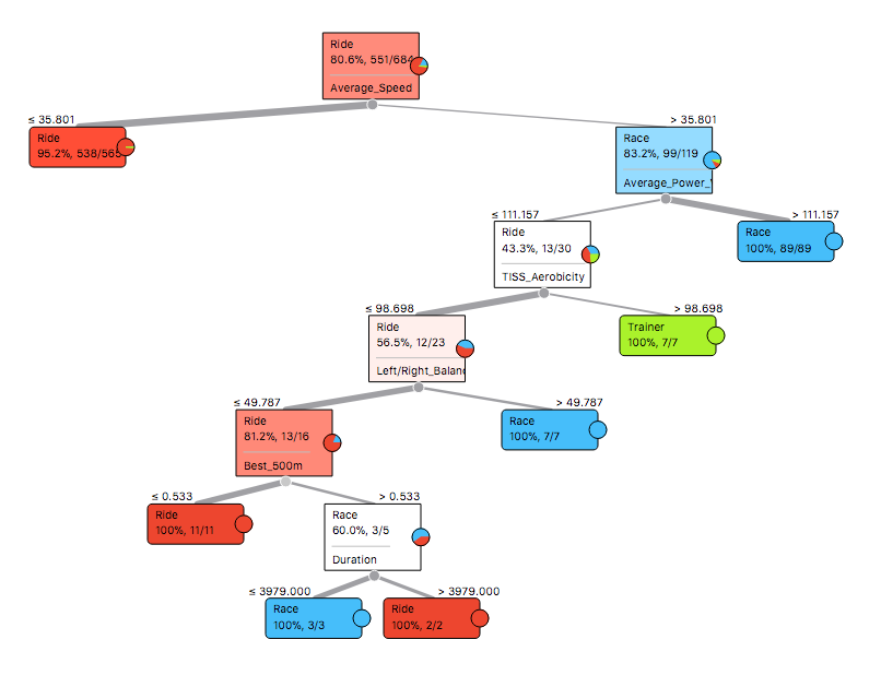
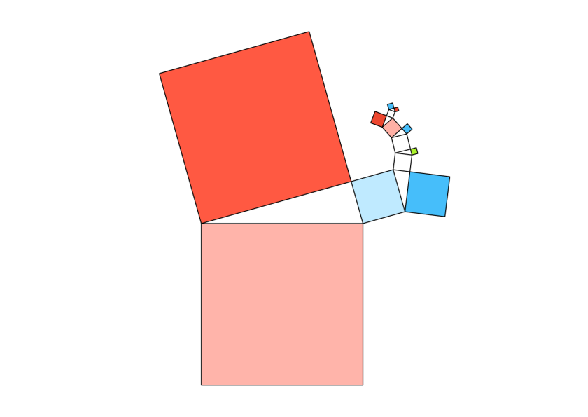
The first split separates the majority of training rides from races and turbo trainer sessions, based on an average speed of 35.8km/h. Then Average Power Variance helped identify races, as observed in the previous blog. After this, turbo trainer sessions seemed to have a high level of TISS Aerobicity, which relates to the percentage of effort done aerobically. Pedalling balance, fastest 500m and duration separated the remaining rides. An attractive way to display these decisions is to create a Pythagorean Tree, where the sides of each triangle relate to the number of observations split by each decision.

Random Forests

Many alternative sets of decisions could separate the data, where any particular tree can be quite sensitive to specific observations. A Random Forest addresses this issue by creating a collection of different decision trees and choosing the class by majority vote. This is the Pythagorean Forest representation of 16 trees, each with six branches.

Support Vector Machines

A Support Vector Machine (SVM) is a widely used model for solving this kind of categorisation problem. The training algorithm finds an efficient way to slice the data, that largely separates the categories, while allowing for some overlap. The points that are closest to the slices are called support vectors. It is tricky to display the results in such a high dimensional space, but the following scatter plot displays Average Power Variance versus Average Speed, where the support vectors are shown as filled circles.

Comparison of results

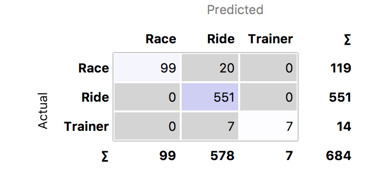
A Confusion Matrix provides a convenient way to compare the accuracy of the models. This correlates the predictions versus the actual category labels. Out of the 809 rides, only 684 were labelled. The Decision Tree incorrectly labelled 20 races and 7 turbos as training rides. The Random Forest did the best job, with only six misclassifications, while the SVM made 11 errors.

Looking at the classification errors can be very informative. It turns out that the two training rides classified as races by the SVM had been accidentally mislabelled – they were in fact races! Furthermore, looking at the five races the that SVM classified as training rides, I punctured in one, I crashed in another and in a third race, I was dropped from the lead group, but eventually rolled in a long way behind with a grupetto. The Random Forest also found an alpine race where my Garmin battery failed and classified it as a training ride. So the misclassifications were largely understandable.

After correcting the data set for mislabelled rides, the Random Forest improved to just two errors and the SVM dropped to just eight errors. The Decision Tree deteriorated to 37 errors, though it did recognise that the climbing rate tends to be zero on a turbo training session.

Prediction

Having trained three models, we can take a look at the sample of 125 unlabelled rides. The following chart shows the predictions of the Random Forest model. It correctly identified one race and suggested several turbo trainer sessions. The SVM also found another race.

Conclusions

Several lessons can be learned from these experiments. Firstly, it is very helpful to start with a clean data set. But if this is not the case, looking at the misclassified results of a decent model can be useful in catching mislabelled data. The SVM seemed to be good for this task, as it had more flexibility to fit the data than the Decision Tree, but it was less prone to overfit the data than the Random Forest.

The Decision Tree was helpful in quickly identifying average speed and power variance (chart below) as the two key variables. The SVM and Random Forest were both pretty good, but less transparent. One might improve on the results by combining these two models.

The next blog will explore this topic further.